MDAnalysis tutorials
Perform post-mortem analysis using Python and MDAnalysis
There are two main ways to analyze data from a molecular dynamics simulation: (1) on-the-fly analysis, for instance using fix ave/time command, and (2) post-mortem analysis, using the trajectories dumped in the lammpstrj file.
The main advantage of post-mortem analysis is that there is no need to know what we want to measure before starting the simulation.
In these short tutorials, several trajectories are imported into Python using MDAnalysis and different information is extracted. All the trajectories required for these tutorials are provided below and were generated from one of the LAMMPS tutorials.
Looking for help or have feedback for us?
Visit the Looking for help? page to get in touch with us.

Simple trajectory import
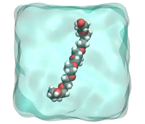
Here, we re-use a trajectory generated during the Polymer in water tutorial. Download the dump and the data files to continue with this tutorial.
Create a Universe
Open a new Jupyter notebook and call it simple_import.ipynb. First, let us import both MDAnalysis and NumPy by copying the following lines into simple_import.ipynb.
import MDAnalysis as mda
import numpy as np
Then, let us create a MDAnalysis universe using the LAMMPS data file mix.data as topology, and the dump.lammpstrj file as trajectory. Add the following lines into the notebook (adapt the path_to_data accordingly):
path_to_data = "./"
u = mda.Universe(path_to_data + "mix.data",
                 path_to_data + "dump.lammpstrj",
                 topology_format="data", format="lammpsdump")
Read topology information
From the Polymer in water tutorial, we know that atom types 1 to 7 are from the PEG atoms, and atom types 8 and 9 are from the water molecules.
One can create atom groups using the atom types with the select_atoms option of MDAnalysis:
peg = u.select_atoms("type 1 2 3 4 5 6 7")
h2o = u.select_atoms("type 8 9")
Let us print the number of atoms in each group:
print("atoms in peg:", peg.atoms.n_atoms)
print("atoms in h2o:", h2o.atoms.n_atoms)
atoms in peg: 101
atoms in h2o: 3045
Atom groups are atom containers, from which information about the atoms can be read. For instance, one can loop over the 6 first atoms from the peg group, and extract their IDs, types, masses, and charges:
for atom in peg[:6]:
    id = atom.id
    type = atom.type
    mass = atom.mass
    charge = np.round(atom.charge,2)
    print("Atom id:", id, "type:", type, "mass:", mass, "g/mol charge:", charge, "e")

Atom id: 3151 type: 4 mass: 1.008 g/mol charge: 0.19 e
Atom id: 3152 type: 6 mass: 15.9994 g/mol charge: -0.31 e
Atom id: 3153 type: 5 mass: 12.011 g/mol charge: 0.06 e
Atom id: 3154 type: 3 mass: 1.008 g/mol charge: 0.05 e
Atom id: 3155 type: 3 mass: 1.008 g/mol charge: 0.05 e
Atom id: 3156 type: 2 mass: 12.011 g/mol charge: 0.02 e
Extract temporal evolution
Let us extract the position of the first atom of the peg group (i.e. the hydrogen of type 4), and store its coordinates in each frame into a list:
atom1 = peg[0]
position_vs_time = []
for ts in u.trajectory:
    x, y, z = atom1.position
    position_vs_time.append([ts.frame, x, y, z])
Here, the for loop runs over all the frames, and the x, y, and z coordinates of the atom named atom1 are read. Here ts.frame is the id of the frame, it goes from 0 to 300, i.e. the total number of frames. The position_vs_time list contains 301 items, each item being the frame id, and the corresponding coordinates of atom1.
One can use Matplotlib Pyplot to visualize all the x and y coordinates occupied by atom1 during the simulation.
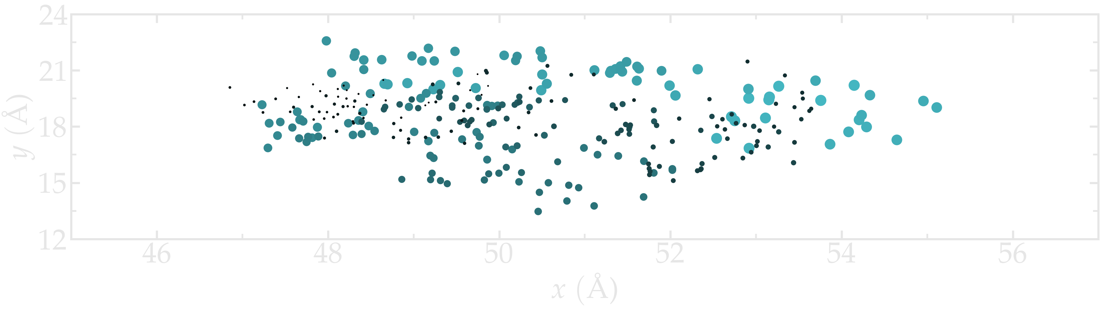
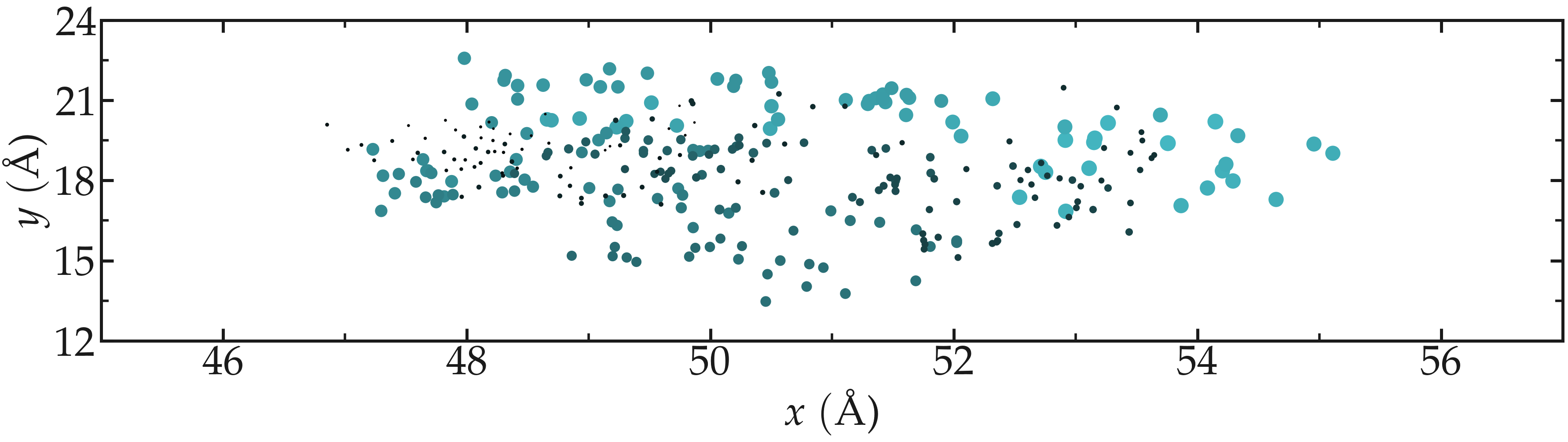
Figure: Position of the atom1 along time. The size of the disks is proportional to the frame ID.
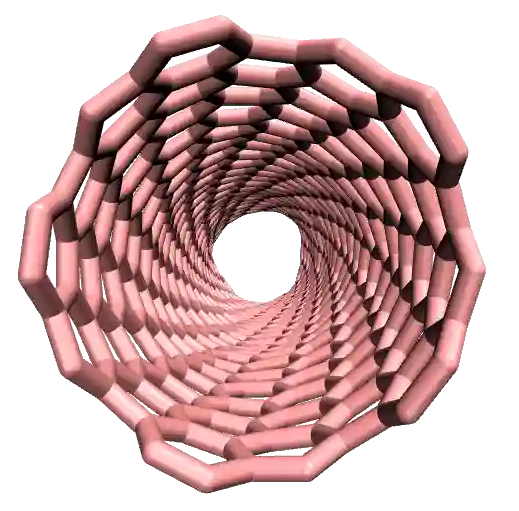
Counting the bonds of a CNT
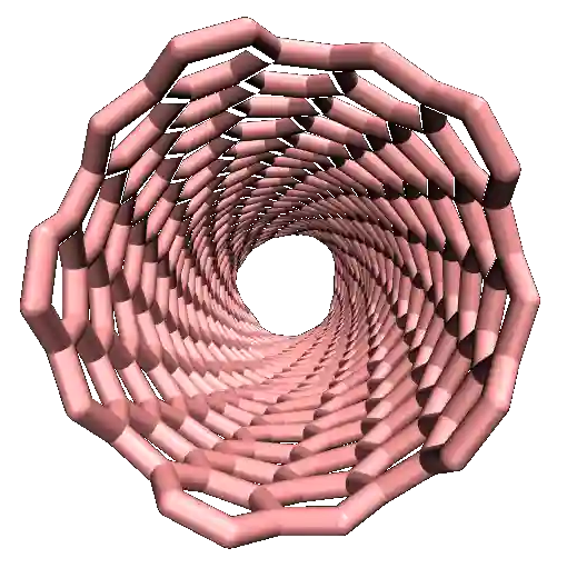
Here, we re-use the trajectory generated during the second part Breakable bonds of the Pulling on a carbon nanotube tutorial. It is recommended that you follow this tutorial first, but you can also directly download the dump file and the data file and continue with this MDA tutorial.
Create a Universe
Open a new Jupyter Notebook and call it measure_bond_evolution.ipynb. First, let us import both MDAnalysis and NumPy by copying the following lines into measure_bond_evolution.ipynb.
import MDAnalysis as mda
import numpy as np
Then, let us create a MDAnalysis universe using the LAMMPS data file cnt_atom.data as topology, and the lammpstrj file as trajectory. Add the following lines into measure_bond_evolution.ipynb:
path_to_data = "./"
u = mda.Universe(path_to_data + "cnt_deformed.data",
                 path_to_data + "dump.lammpstrj",
                 topology_format="data", format="lammpsdump",
                 atom_style='id type xs ys zs',
                 guess_bonds=True, vdwradii={'1':1.7})
Since the .data file does not contain any bond information the original bonds are guessed using the bond guesser of MDAnalysis using guess_bonds=True.
Note that the bond guesser of MDAnalysis will not update the list of bond over time, so we will need to use a few tricks to extract the evolution of the number of bonds with time.
Let us create a single-atom group named cnt and containing all the carbon atoms, i.e. all the atoms of type 1, by adding the following lines into measure_bond_evolution.ipynb.
cnt = u.select_atoms("type 1")
Some basics of MDAnalysis
MDAnalysis allows us to easily access information concerning the simulation, such as the number of atoms, or the number of frames in the trajectory:
print("Number of atoms =", cnt.n_atoms)
print("Number of frames =", u.trajectory.n_frames)

Number of atoms = 690
Number of frames = 286
It is also possible to access the indexes of the atoms that are considered as bonded by the bond guesser of MDAnalysis:
print(cnt.atoms.bonds.indices)

[[  0   2]
[  0  23]
[  0  56]
(...)
[686 687]
[686 689]
[688 689]]
MDAnalysis also offers the possibility to loop over all the frame of the trajectory using:
for ts in u.trajectory:
    print(ts.frame)

0
1
2
3
(...)
283
284
285
The positions of the atoms can also be obtained using:
u.atoms.positions

array([[ 75.14728 ,  78.17872 ,  95.61408 ],
[ 75.33008 ,  77.751114,  93.20232 ],
[ 75.550476,  77.34152 ,  94.54224 ],
...,
[ 84.66992 ,  82.24888 , 143.84988 ],
[ 84.66992 ,  82.24888 , 147.60156 ],
[ 84.85272 ,  81.82128 , 146.26175 ]], dtype=float32)
where the three columns of the array are the x, y, and z coordinates of the atoms.
Counting the bonds
In order to measure the evolution of the number of bonds over time, let us loop over the trajectory and manually extract the inter-atomic distance over time.
To do so, for every step of the trajectory, let us loop over the indexes of the atoms that were initially detected as bonded, and calculate the distance between the two atoms, which can be done using:
for ts in u.trajectory:
    for id1, id2 in cnt.atoms.bonds.indices:
        # detect positions
        pos1 = u.atoms.positions[u.atoms.indices == id1][0]
        pos2 = u.atoms.positions[u.atoms.indices == id2][0]
        r = np.sqrt(np.sum((pos1-pos2)**2))
Then, let us assume that if \(r\) is larger that a certain cut-off value of, let’s say, \(1.8\,Å\), the bond is broken:
for ts in u.trajectory:
    for id1, id2 in cnt.atoms.bonds.indices:
        pos1 = u.atoms.positions[u.atoms.indices == id1][0]
        pos2 = u.atoms.positions[u.atoms.indices == id2][0]
        r = np.sqrt(np.sum((pos1-pos2)**2))
        if r < 1.8:
            print("the bond has a length", r, "Å")
        else:
            print("the bond is broken")
Finally, let us store both the mean length of the bonds and the total number of bonds in lists.
lbond_vs_frame = []
nbond_vs_frame = []
for ts in u.trajectory:
    frame = ts.frame
    all_bonds_ts = [] # temporary list to store bond length
    for id1, id2 in cnt.atoms.bonds.indices:
        pos1 = u.atoms.positions[u.atoms.indices == id1]
        pos2 = u.atoms.positions[u.atoms.indices == id2]
        r = np.sqrt(np.sum((pos1-pos2)**2))
        if r < 1.8:
            all_bonds_ts.append(r)
    mean_length_bonds = np.mean(all_bonds_ts)
    number_of_bond = len(all_bonds_ts)/2 # divide by 2 to avoid counting twice
    lbond_vs_frame.append([frame, mean_length_bonds])
    nbond_vs_frame.append([frame, number_of_bond])
The data can then be saved to files:
np.savetxt("number_bond_vs_time.dat", nbond_vs_frame)
np.savetxt("length_bond_vs_time.dat", lbond_vs_frame)
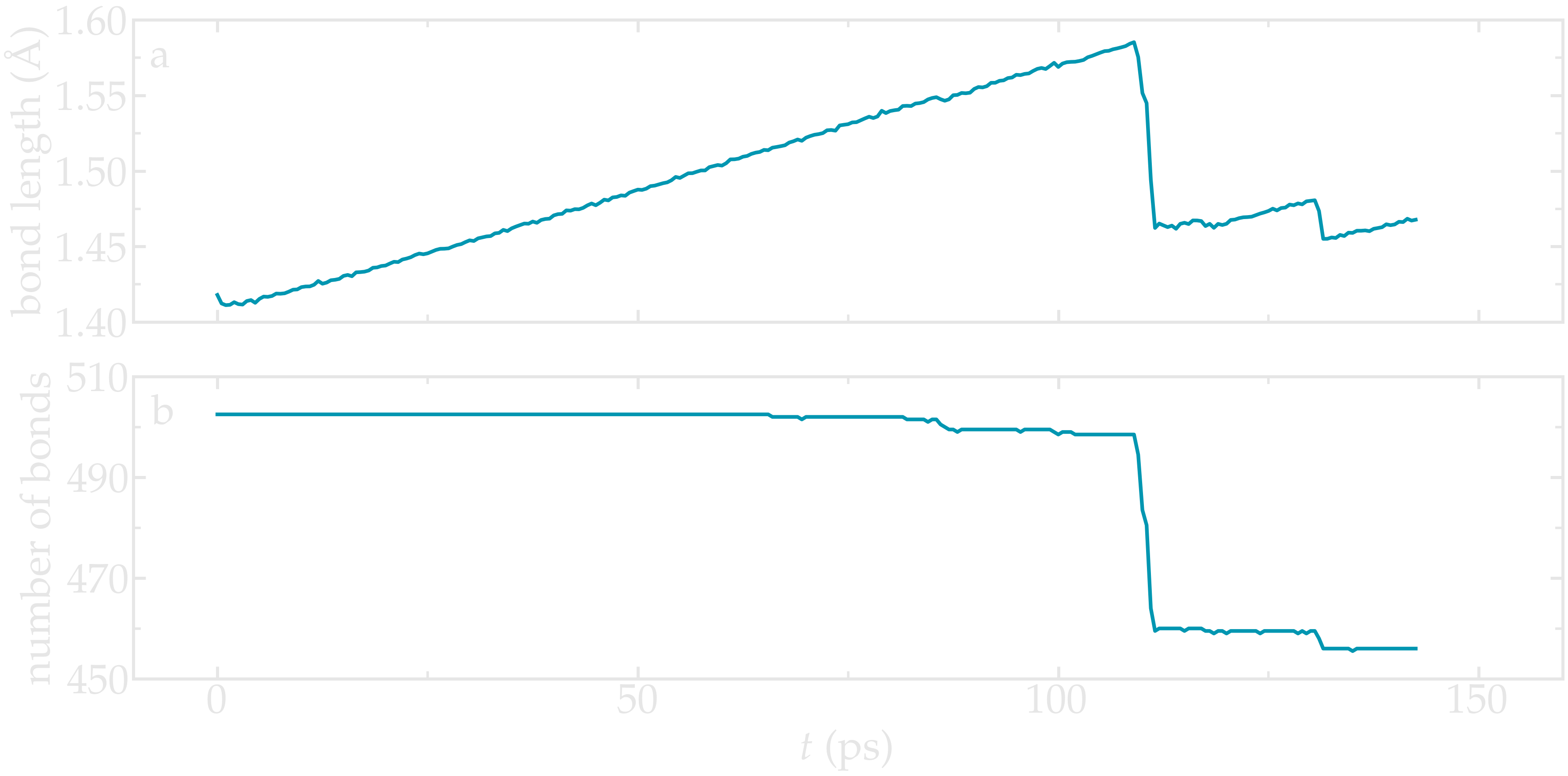
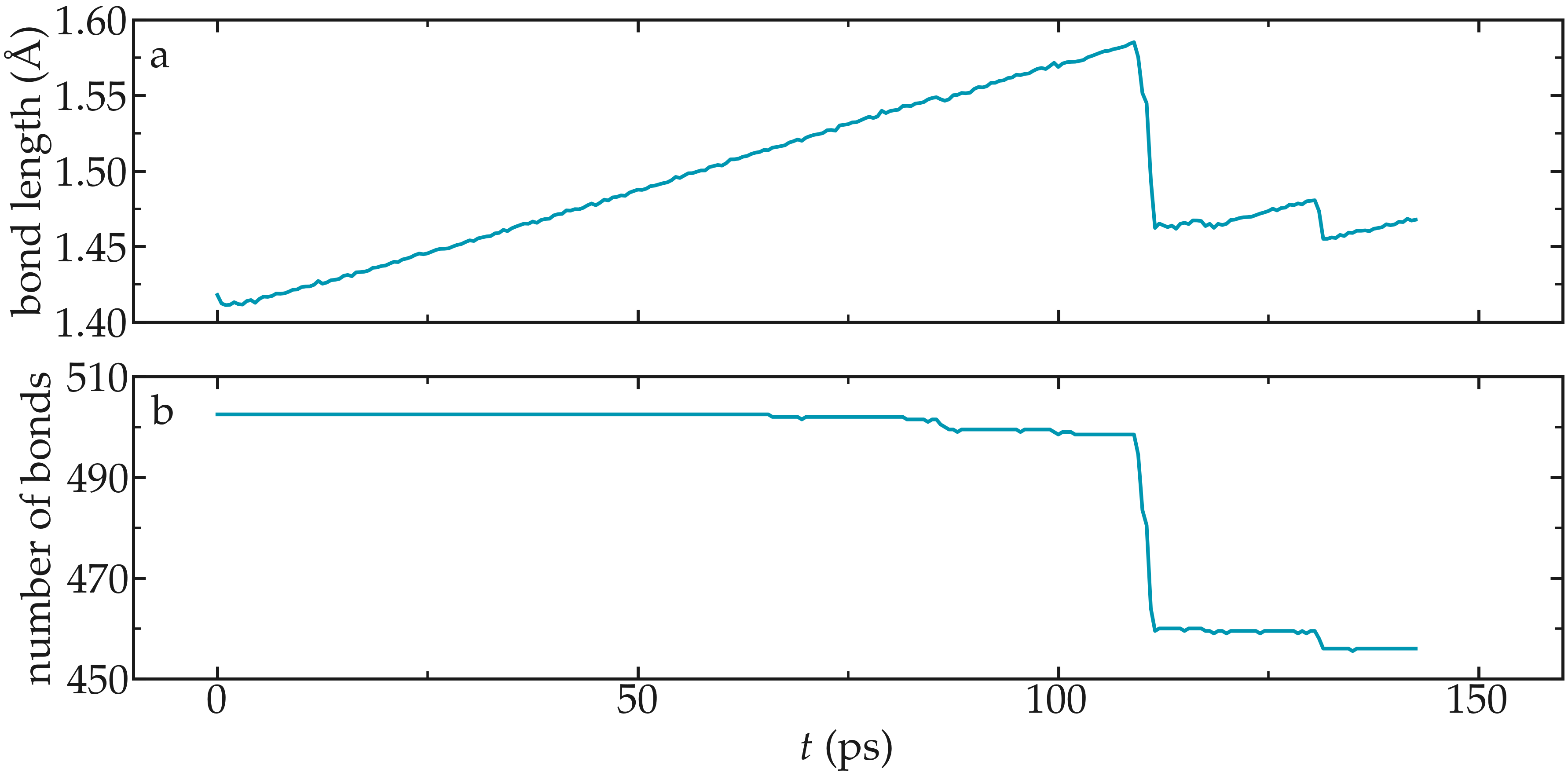
Figure: Evolution of the average bond length (a) and bond number (b) as a function of time.
Bond length distributions
Using a similar script, let us extract the bond length distribution at the beginning of the simulation (let us say the 20 first frame), as well as near the maximum deformation of the CNT:
bond_length_distributions = []
for ts in u.trajectory:
    all_bonds_ts = []
    for id1, id2 in cnt.atoms.bonds.indices:
        pos1 = u.atoms.positions[u.atoms.indices == id1]
        pos2 = u.atoms.positions[u.atoms.indices == id2]
        r = np.sqrt(np.sum((pos1-pos2)**2))
        if r < 1.8:
            all_bonds_ts.append(r)
    if frame > 0: # ignore the first frame
        histo, r_val = np.histogram(all_bonds_ts, bins=50, range=(1.3, 1.65))
        r_val = (r_val[1:]+r_val[:-1])/2
        bond_length_distributions.append(np.vstack([r_val, histo]))
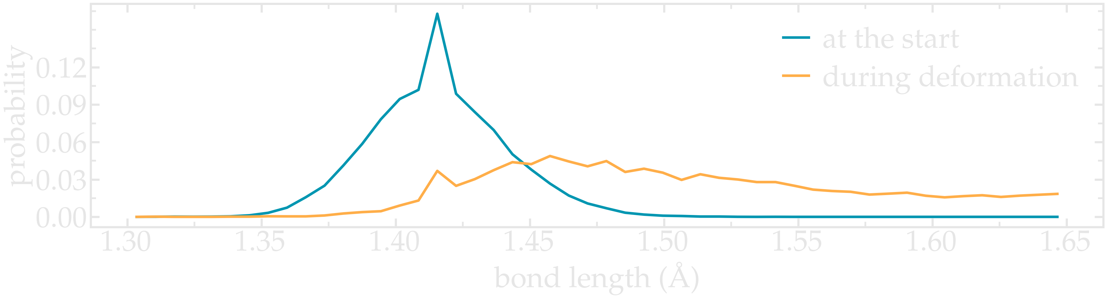
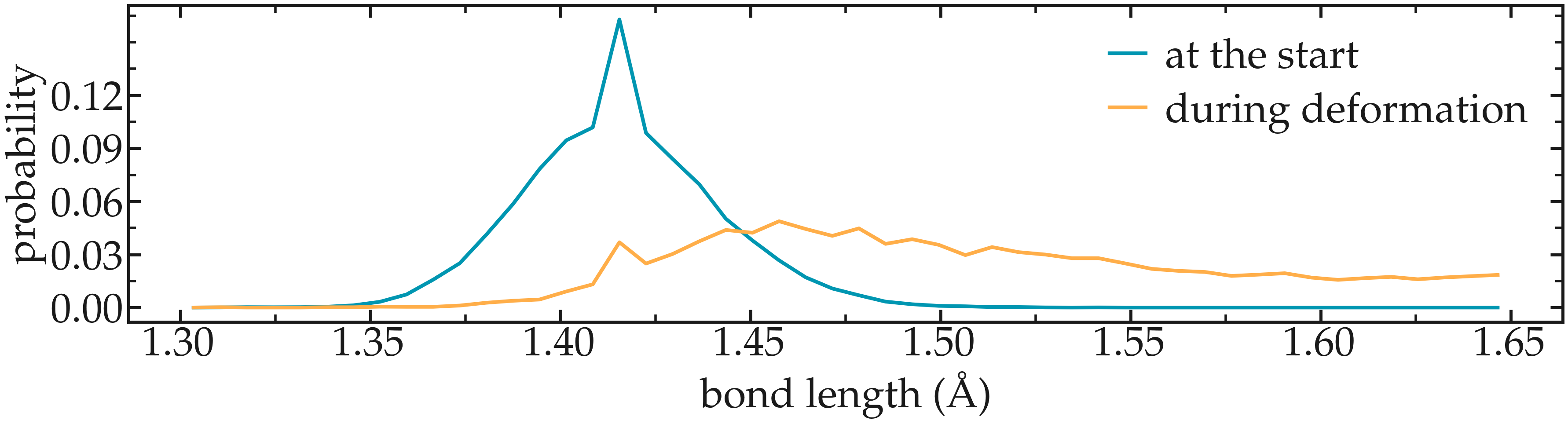
Figure: Distribution in bond length near the start of the simulation, as well as near the maximum deformation of the CNT.