Solutions to the exercises

Lennard Jones fluid

Fix a broken input

A possibility to make the simulation start without error is to reduce the initial timestep value as well as the imposed temperature. You can download the working input I wrote. These are the main commands:

fix mylgv all langevin 0.001 0.001 0.001 1530917
timestep 0.0001

Note that to make sure that the temperature of the particles quickly reaches a reasonable value, the damping parameter of the fix Langevin was also reduced to 0.001 (in time units) instead of the 0.1 used in the rest of the tutorial.

After the first run finishes, the energy of the system should be significantly reduced. Therefore, a second consecutive run with the original timestep and Langevin parameters can start without triggering the Lost atoms error.

In some cases, more than two consecutive runs with progressively increasing timestep is necessary:

fix mylgv all langevin 0.0001 0.0001 0.001 1530917
timestep 0.0001
run 10000

timestep 0.001
run 10000

timestep 0.01
run 10000

An alternative solution was proposed by Joni Suopanki from the University of Oulu in Finland. His solution consists of making the LJ potential softer by using small values for \(\sigma_{11}\), as least during the very first steps of the simulation:

pair_coeff 1 1 1.0 0.5
run 1
pair_coeff 1 1 1.0 0.75
run 1
pair_coeff 1 1 1.0 1.0
run 10000

Create a demixed dense phase

You can download the input I wrote. Note that I use large numbers of particles: 8000 for each type.

The key to creating a demixing phase is to find the appropriate Lennard-Jones parameters:

pair_coeff 1 1 5.0 1.0
pair_coeff 2 2 5.0 1.0
pair_coeff 1 2 0.05 1.0

Here, both particle types have the same \(\sigma\) value of 1.0 so that both particles have the same diameter. There is a large energy parameter \(\epsilon_{11} = \epsilon_{22} = 5.0\) for self-interaction (i.e. interaction between particles of the same type), and a low energy parameter \(\epsilon_{12} = 0.05\) for interaction between particles of different types.

Finally, to easily adjust the system density and create a liquid-looking phase, the pressure was imposed by replacing fix nve by fix nph:

fix mynph all nph iso 1.0 1.0 1.0

With fix nph and a pressure of 1, LAMMPS adjusts the box dimensions until the pressure is close to 1. Here, reaching a pressure of 1 requires reducing the initial box dimensions.

From atoms to molecules

You can download an example of input for simulating dumbell molecules.

The first important change to make to the inputs from the tutorial is the atom_style: an atom_style that allows for the atoms to be connected by bonds is needed. It is also necessary to specify the bond_style, i.e. the type of potential (here harmonic) that will keep the atoms together:

atom_style molecular
bond_style harmonic

When creating the box, it is necessary to make memory space for the bond:

create_box 2 simulation_box bond/types 1 extra/bond/per/atom 1

Then, one just needs to import the molecule template, and use the template when creating the atoms as follows:

molecule dumbell dumbell.mol
create_atoms 1 random 500 341341 simulation_box
create_atoms 0 random 5 678865 simulation_box mol dumbell 8754

You can download the molecule template by clicking here. Finally, some parameters for the bond, namely its rigidity (5) and equilibrium length (2.5) need to be specified:

bond_coeff 1 5 2.5

For the polymer, the angular potential must be defined to give its rigidity to the polymer. You can download the input and molecule template.

Pulling on a carbon nanotube

Plot the strain-stress curves

You can download the input for the breakable CNT and input for the unbreakable CNT I wrote.

The stress is calculated as the total force induced on the CNT by the pulling divided by the surface area of the CNT.

On a side note, the surface area of a CNT is not a well-defined quantity. Here, I choose to define the area as the perimeter of the CNT multiplied by the effective width of the carbon atoms.

Be careful with units, as the force is either in kcal/mol/Å when the unit is real, i.e. for the unbreakable CNT, or in eV/Å when the unit is metal, i.e. for the breakable CNT.

Solve the flying ice cube artifact

The issue occurs because the atoms have a large momentum in the \(x\) direction, as can be seen by looking at the net velocity of the atoms in the cnt_molecular.data file.

Velocities

24 0.007983439029626362 -6.613056392124822e-05 7.867644943646289e-05
1 0.007906200203484036 3.252025147011299e-05 -4.4209216231039336e-05
25 0.007861090484107148 9.95045322688365e-06 -0.00014277147407215768
(...)

The Berendsen thermostat is trying to adjust the temperature of the system by rescaling the velocity of the atoms, but fails due to the large momentum of the system that makes it look like the system is warm, since in MD temperature is measured from the kinetic energy.

This leads to the system appearing frozen.

The solution is to cancel the net momentum of the atoms, for instance by using fix momentum, re-setting the velocity with the velocity create command, or use a different thermostat.

Insert gas in the carbon nanotube

You can download the input I wrote.

The key is to modify the .data file to make space for the second atom type 2.

670 impropers
2 atom types
1 bond types

(...)

Masses

1 12.010700 # CA
2 39.948 # Ar

The parm.lammps must contain the second pair coeff:

pair_coeff 1 1 0.066047 3.4
pair_coeff 2 2 0.232 3.3952
bond_coeff 1 469 1.4

Combine the region and create_atoms commands to create the atoms of type 2 within the CNT:

region inside_CNT cylinder z 0 0 2.5 ${zmin} ${zmax}
create_atoms 2 random 40 323485 inside_CNT overlap 1.8 maxtry 50

It is good practice to thermalize the CNT separately from the gas to avoid having a large temperature difference between the two type of atoms.

compute tcar carbon_atoms temp
fix myber1 all temp/berendsen ${T} ${T} 100
fix_modify myber1 temp tcar
compute tgas gas temp
fix myber2 all temp/berendsen ${T} ${T} 100
fix_modify myber2 temp tgas

Here I also choose to keep the CNT near its original position,

fix myspr carbon_atoms spring/self 5

Make a membrane of CNTs

You can download the input I wrote.

The CNT can be replicated using the replicate command. It is recommended to adjust the box size before replicating, as done here using the change_box command.

To allow for the deformation of the box along the xy plane, the box has to be changed to triclinic first:

change_box all triclinic

Deformation can be imposed to the system using:

fix muyef all deform 1 xy erate 5e-5

Polymer in water

Extract radial distribution function

You can download the input file I wrote.

I use the compute rdf command of LAMMPS to extract the RDF between atoms of type 8 (oxygen from water) and one of the oxygen types from the PEG (1). The 10 first pico seconds are disregarded. Then, once the force is applied to the PEG, a second fix ave/time is used.

compute myRDF_PEG_H2O all rdf 200 1 8 2 8 cutoff 10
fix myat2 all ave/time 10 4000 50000 c_myRDF_PEG_H2O[*] &
    file PEG-H2O-initial.dat mode vector

Add salt to the mixture

You can download the input, data, and parm files I wrote.

It is important to make space for the two salt atoms by modifying the data file as follows:

(...)
11 atom types
(...)

Additional mass and pair_coeff lines must also be added to the parm file (be careful to use the appropriate units):

(...)
mass 10 22.98 # Na
mass 11 35.453 # Cl
(...)
pair_coeff 10 10 0.04690 2.43 # Na
pair_coeff 11 11 0.1500 4.045
(...)

Finally, here I choose to add the ions using two separate create_atoms commands with a very small overlap values, followed by an energy minimization.

Note also the presence of the set commands to give a net charge to the ions.

Evaluate the deformation of the PEG

You can download the input file I wrote.

The key is to combine the compute dihedral/local, which computes the angles of the dihedrals and returns them in a vector, with the ave/histo functionalities of LAMMPS:

compute mydihe all dihedral/local phi
fix myavehisto all ave/histo 10 2000 30000 0 180 500 c_mydihe &
    file initial.histo mode vector

Here I choose to unfix myavehisto at the end of the first run, and to re-start it with a different file name during the second phase of the simulation.

Nanosheared electrolyte

Induce a Poiseuille flow

Here, the input script written during the last part Imposed shearing of the tutorial is adapted so that, instead of a shearing induced by the relative motion of the walls, the fluid motion is generated by an additional force applied to both water molecules and ions.

To do so, here are the most important commands used to properly thermalize the system:

fix mynve all nve
compute tliq fluid temp/partial 0 1 1
fix myber1 fluid temp/berendsen 300 300 100
fix_modify myber1 temp tliq
compute twall wall temp
fix myber2 wall temp/berendsen 300 300 100
fix_modify myber2 temp twall

Here, since walls wont move, they can be thermalized in all 3 directions and there is no need for recentering. Instead, one can keep the walls in place by adding springs to every atom:

fix myspring wall spring/self 10.0 xyz

Finally, let us apply a force to the fluid group along the \(x\) direction:

fix myadf fluid addforce 3e-2 0.0 0.0

The choice of a force equal to \(f = 0.03\,\text{kcal/mol/Å}\) is discussed below.

One can have a look at the velocity profiles. The fluid shows the characteristic parabolic shape of Poiseuille flow in the case of a non-slip solid surface. To obtain smooth-looking data, I ran the simulation for a total duration of \(1\,\text{ns}\). To lower the duration of the computation, don’t hesitate to use a shorter duration like \(100\,\text{ps}\).

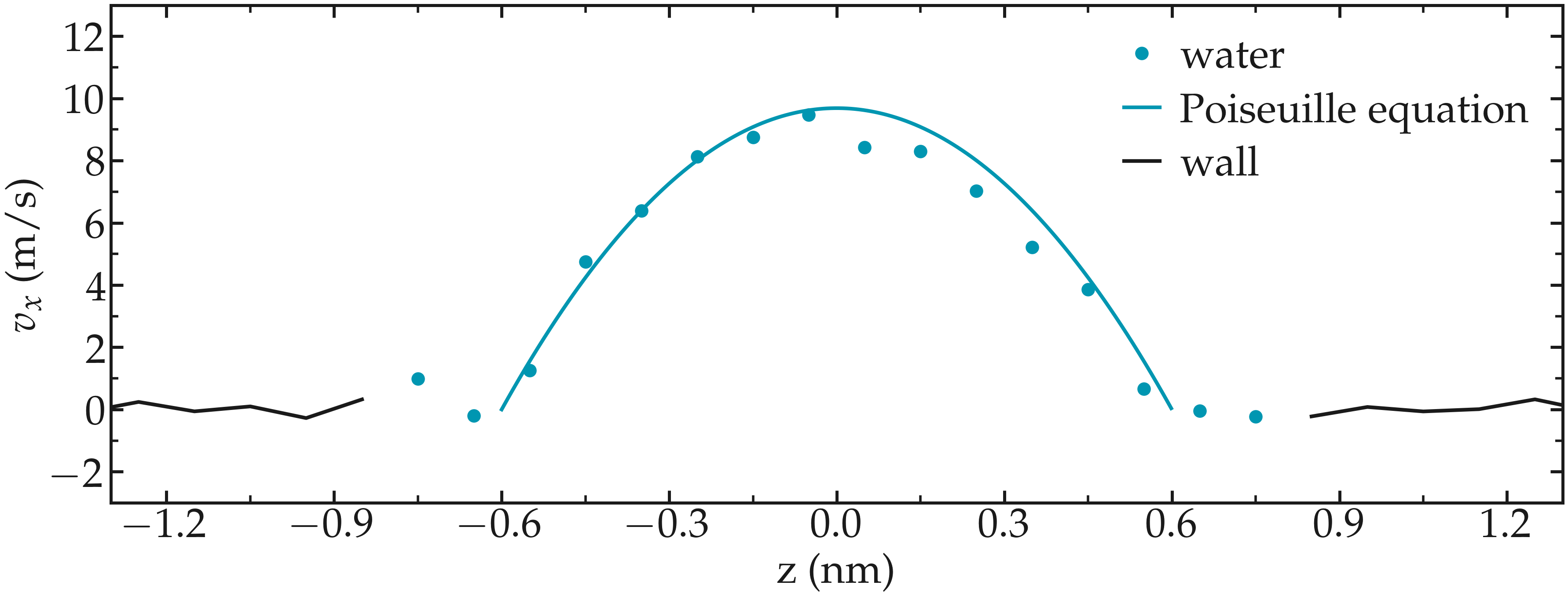
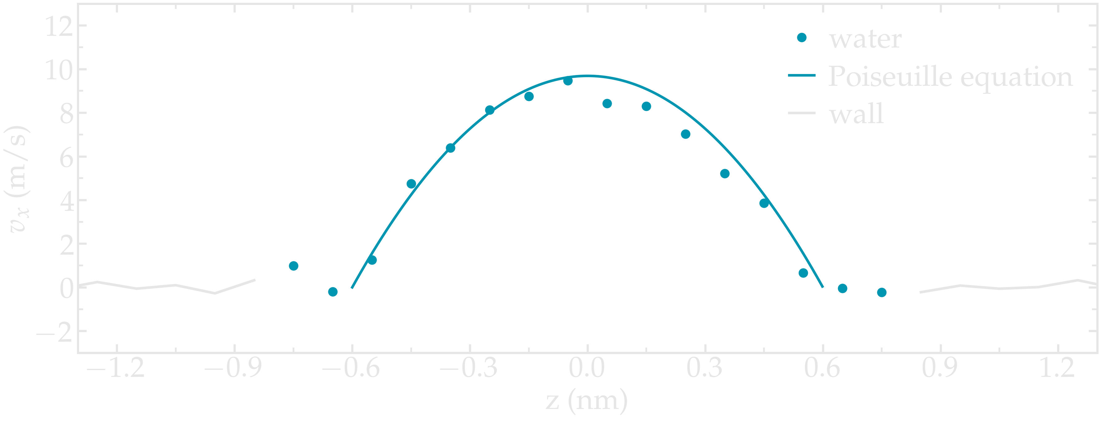
Figure: Velocity profiles of the water molecules along the z axis (disks). The line is the Poiseuille equation.

The fitting of the velocity profile was made using the following Poiseuille equation,

\[v = - \alpha \dfrac{f \rho}{\eta} \left( \dfrac{z^2}{2} - \dfrac{h^2}{8} \right),\]

where \(\textbf{f}\) is the applied force, \(\rho\) is the fluid density, \(\eta\) is the fluid viscosity, and \(h = 1.2\,\text{nm}\) is the pore size. The expression for \(v\) can be derived from the Stokes equation \(\eta \nabla \textbf{v} = - \textbf{f} \rho\). A small correction \(\alpha = 0.78\) was necessary, since using bulk density and bulk viscosity is obviously not correct in such nanoconfined pores. More subtle corrections could be applied by correcting both density and viscosity based on independent measurements, but this is beyond the scope of the present exercise.

Choosing the right force

The first and most important technical difficulty of any out-of-equilibrium simulation is to choose the value of the force \(f\). If the forcing is too large, the system may not be in a linear response regime, meaning that the results are forcing-dependent (and likely quite meaningless). If the forcing is too small, the motion of the system will be difficult to measure due to the low signal-to-noise ratio.

In the present case, one can perform a calibration by running several simulations with different force values \(f\), and then by plotting the velocity of the center of mass \(v_\text{cm}\) of the fluid as a function of the force. Here, I present the results I have obtained by performing the simulations with different values of the forcing. \(v_\text{cm}\) can be extracted by adding the following command to the input:

variable vcm_fluid equal vcm(fluid,x)
fix myat1 all ave/time 10 100 1000 v_vcm_fluid file vcm_fluid.dat

The results show that as long as the force is lower than about \(0.04\,\text{kcal/mol/Å}\), there is reasonable linearity between force and fluid velocity.

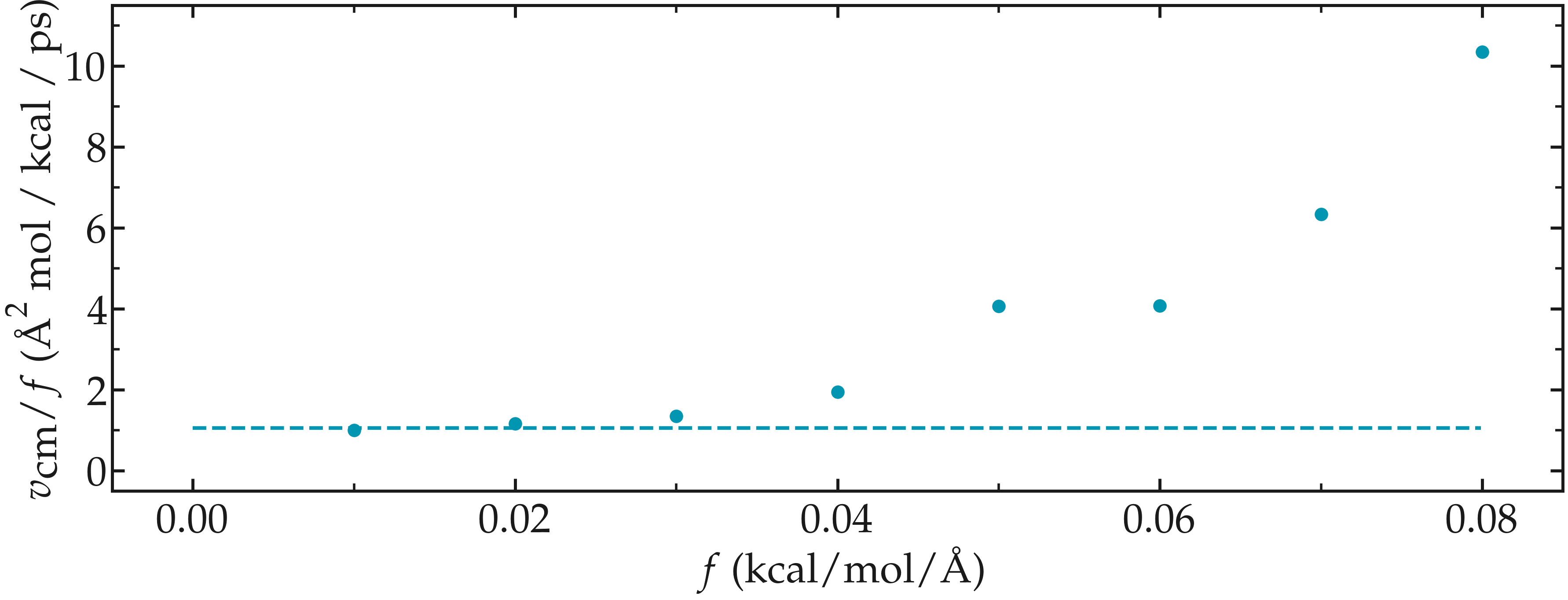
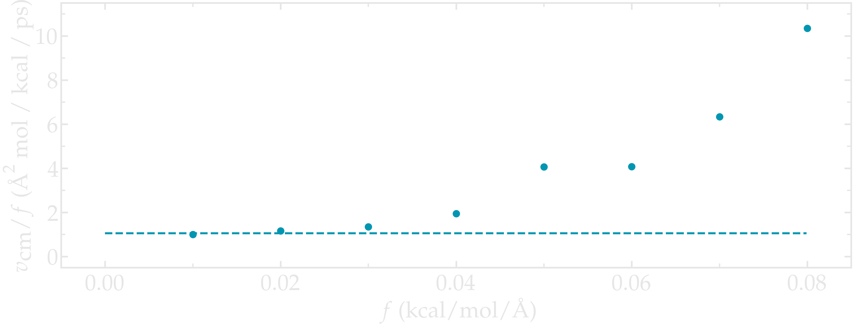
Figure: Ratio between the velocity of the center of mass \(v_\text{cm}\) of the fluid and the force \(f\) as a function of the forcing

Water adsorption in silica

Mixture adsorption

You can download the input for the combine water and CO2 adsorption. One of the first steps is to create both types of molecules before starting the GCMC:

molecule h2omol H2O.mol
molecule co2mol CO2.mol
create_atoms 0 random 5 456415 NULL &
    mol h2omol 454756 overlap 2.0 maxtry 50
create_atoms 0 random 5 373823 NULL &
    mol co2mol 989812 overlap 2.0 maxtry 50

One must be careful to properly write the parameters of the system, with all the proper cross coefficients:

pair_coeff * * vashishta ../../Potential/SiO.1990.vashishta &
    Si O NULL NULL NULL NULL
pair_coeff * * lj/cut/tip4p/long 0 0
pair_coeff 1 3 lj/cut/tip4p/long 0.0057 4.42
pair_coeff 1 5 lj/cut/tip4p/long 0.01096 3.158
pair_coeff 1 6 lj/cut/tip4p/long 0.007315 3.2507
pair_coeff 2 3 lj/cut/tip4p/long 0.0043 3.12
pair_coeff 2 5 lj/cut/tip4p/long 0.0101 2.858
pair_coeff 2 6 lj/cut/tip4p/long 0.0065 2.9512
pair_coeff 3 3 lj/cut/tip4p/long 0.008 3.1589
pair_coeff 3 5 lj/cut/tip4p/long 0.01295 2.8924
pair_coeff 3 6 lj/cut/tip4p/long 0.0093 2.985
pair_coeff 4 4 lj/cut/tip4p/long 0.0 0.0
pair_coeff 5 5 lj/cut/tip4p/long 0.0179 2.625854
pair_coeff 6 6 lj/cut/tip4p/long 0.0106 2.8114421

Here, I choose to thermalize all species separately:

compute ctH2O H2O temp
compute_modify ctH2O dynamic yes
fix mynvt1 H2O nvt temp 300 300 0.1
fix_modify mynvt1 temp ctH2O

compute ctCO2 CO2 temp
compute_modify ctCO2 dynamic yes
fix mynvt2 CO2 nvt temp 300 300 0.1
fix_modify mynvt2 temp ctCO2

compute ctSiO SiO temp
fix mynvt3 SiO nvt temp 300 300 0.1
fix_modify mynvt3 temp ctSiO

Finally, adsorption is made with two separate fix gcmc commands placed in a loop:

label loop
variable a loop 30

fix fgcmc_H2O H2O gcmc 100 100 0 0 65899 300 -0.5 0.1 &
    mol h2omol tfac_insert ${tfac} group H2O shake shak &
    full_energy pressure 100 region system
run 500
unfix fgcmc_H2O

fix fgcmc_CO2 CO2 gcmc 100 100 0 0 87787 300 -0.5 0.1 &
    mol co2mol tfac_insert ${tfac} group CO2 &
    full_energy pressure 100 region system
run 500
unfix fgcmc_CO2

next a
jump SELF loop

Here I choose to apply the first fix gcmc for the \(\text{H}_2\text{O}\) for 500 steps, then unfix it before starting the second fix gcmc for the \(\text{CO}_2\) for 500 steps as well. Then, thanks to the jump, these two fixes are applied successively 30 times each, allowing for the progressive adsorption of both species.

Adsorb water in ZIF-8 nanopores

You can download the input for the water adsorption in Zif-8, which you have to place in the same folder as the zif-8.data, parm.lammps, and water.mol files.

Apart from the parameters and topology, the input is quite similar to the one developed in the case of the crack silica.

You should observe an increase in the number of molecules with time. Run a much longer simulation if you want to saturate the porous material with water.

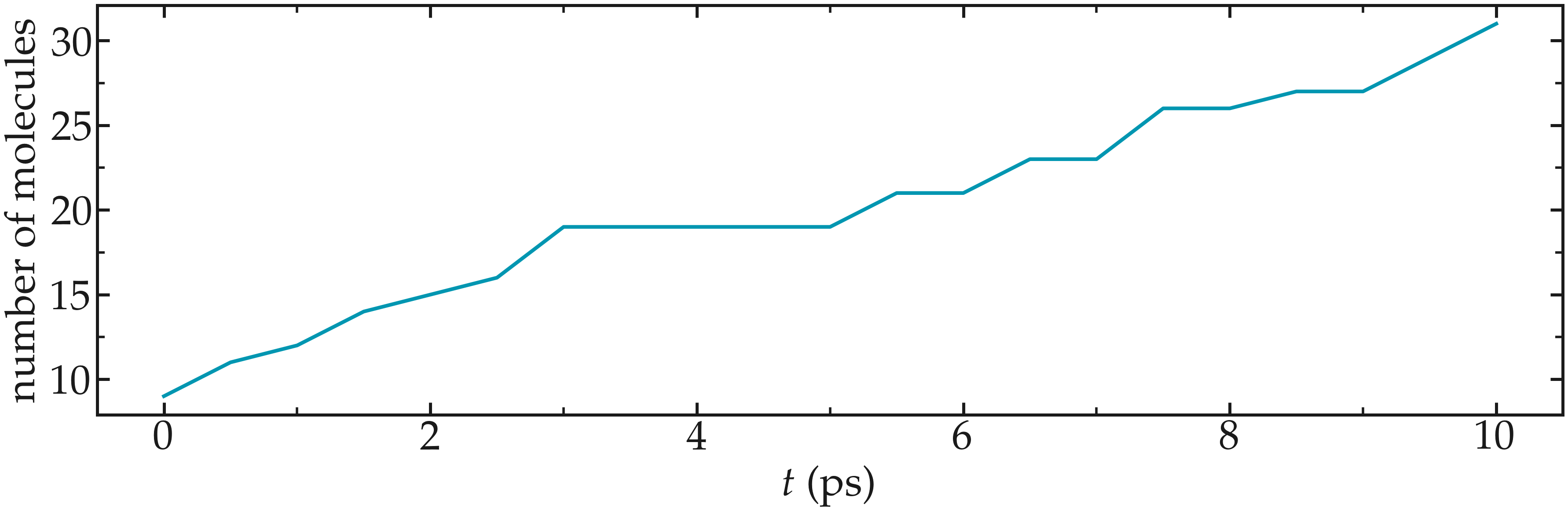
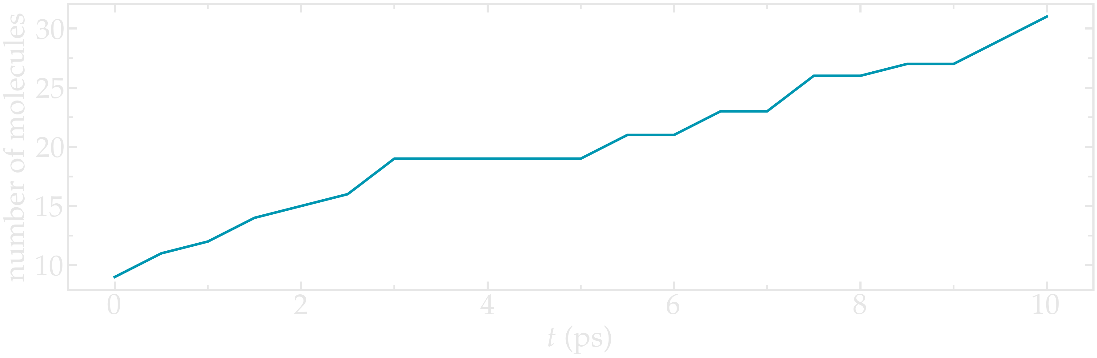
Figure: Number of water molecules in Zif-8 during the first \(10\,ps\).

Free energy calculation

The binary fluid that won’t mix

You can download the input here.

The solution chosen here was to create two groups (t1 and t2) and apply the two potentials U1 and U2 to each group, respectively.

To to so, two separate fix addforce are used:

group t1 type 1
variable U1 atom ${U0}*atan((x+${x0})/${dlt}) &
    -${U0}*atan((x-${x0})/${dlt})
variable F1 atom ${U0}/((x-${x0})^2/${dlt}^2+1)/${dlt} &
    -${U0}/((x+${x0})^2/${dlt}^2+1)/${dlt}
fix myadf1 t1 addforce v_F1 0.0 0.0 energy v_U1
fix_modify myadf1 energy yes

group t2 type 2
variable U2 atom -${U0}*atan((x+${x0})/${dlt}) &
    +${U0}*atan((x-${x0})/${dlt})
variable F2 atom -${U0}/((x-${x0})^2/${dlt}^2+1)/${dlt} &
    +${U0}/((x+${x0})^2/${dlt}^2+1)/${dlt}
fix myadf2 t2 addforce v_F2 0.0 0.0 energy v_U2
fix_modify myadf2 energy yes

60 particles of each type are created, with both types having the same properties:

mass * 39.95
pair_coeff * * ${epsilon} ${sigma}

Feel free to insert some size or mass asymmetry in the mixture, and test how/if it impacts the final potential.

Particles under convection

Add a forcing to all the particles using:

fix myconv all addforce 2e-6 0 0

It is crucial to choose a forcing that is not too large, or the simulation may crash. A forcing that is too weak won’t have any effect on the PMF.

One can see from the result that the measured potential is tilted, which is a consequence of the additional force that makes it easier for the particles to cross the potential in one of the directions. The barrier is also reduced compared to the case in the absence of additional forcing.

Surface adsorption of a molecule

You can download the input here.

Reactive silicon dioxide

Hydrate the structure

See the input here, and create a molecule template named H2O.mol:

3 atoms

Coords

1    0 0 0
2    0.9584 0 0
3    -0.23996 0.92787 0

Types

1        2
2        3
3        3

Charges

1       -1.1128
2        0.5564
3        0.5564

Add molecules to the system using:

molecule h2omol H2O.mol
create_atoms 0 random 10 805672 NULL overlap 2.6 maxtry 50 mol h2omol 45585

One can see that some water molecules have reacted during the simulation:

#  Timestep No_Moles No_Specs Si192O384H20 OH2
   5        21       2        1            20

#  Timestep No_Moles No_Specs Si192O387H26 OH2 OH3 O2H3
   10000    17       4        1            14  1   1

A slightly acidic bulk solution

See the input here, and create a molecule template named H2O.mol:

3 atoms

Coords

1    0 0 0
2    0.9584 0 0
3    -0.23996 0.92787 0

Types

1        1
2        2
3        2

Charges

1       -1.1128
2        0.5564
3        0.5564

Here, apart from creating water molecules everywhere in the box, a few additional hydrogen atoms are added randomly to the system to make the solution slightly acidic.