Nanosheared electrolyte
Aqueous NaCl solution sheared by two walls
The objective of this tutorial is to simulate an electrolyte nanoconfined and sheared by two walls. The density and velocity profiles of the fluid in the direction normal to the walls are extracted to highlight the effect of confining a fluid on its local properties.
This tutorial illustrates some key aspects of combining a fluid and a solid in the same simulation. A major difference from Polymer in water is that here a rigid four-points water model named TIP4P is used [36]. TIP4P is one of the most common water models due to its high accuracy.
If you are completely new to LAMMPS, I recommend that you follow this tutorial on a simple Lennard-Jones fluid first.
If you find these tutorials useful for your research or simulations, you can cite: A Set of Tutorials for the LAMMPS Simulation Package by Simon Gravelle, Jacob R. Gissinger, and Axel Kohlmeyer (2025) [13]. You can access the full paper on arXiv.
This tutorial is compatible with the 2Aug2023 LAMMPS version.
System preparation
The fluid and walls must first be generated and then equilibrated at a reasonable temperature and pressure.
System generation
Create a new folder called systemcreation/. Within systemcreation/, open a blank file called input.lammps, and copy the following lines into it:
boundary p p f
units real
atom_style full
bond_style harmonic
angle_style harmonic
pair_style lj/cut/tip4p/long 1 2 1 1 0.1546 12.0
kspace_style pppm/tip4p 1.0e-4
kspace_modify slab 3.0
These lines are used to define the most basic parameters, including the atom, bond, and angle styles, as well as interaction potential. Here, lj/cut/tip4p/long imposes a Lennard Jones potential with a cut-off at \(12\,\text{Å}\) and a long-range Coulomb potential.
So far, the commands are relatively similar to those in the previous tutorial, Polymer in water, with two major differences: the use of lj/cut/tip4p/long instead of lj/cut/coul/long, and pppm/tip4p instead of pppm. These two tip4p-specific commands allow us to model a four-point water molecule without explicitly defining the fourth massless atom M. The value of \(0.1546\,\text{Å}\) corresponds to the O-M distance and is imposed by the water model. Here, TIP4P-2005 is used [36].
Another novelty, here, is the use of kspace_modify slab 3.0 that is combined with the non-periodic boundaries along the z coordinate: boundary p p f. With the slab option, the system is treated as periodical along z, but with an empty volume inserted between the periodic images of the slab, and the interactions along z effectively turned off.
About lj/cut/tip4p/long pair style
The lj/cut/tip4p/long pair style is similar to the conventional Lennard Jones and Coulomb interactions, except that it is specifically designed for four-point water model (tip4p). The atoms of the water model will be type 1 (O) and 2 (H). All the other atoms in the simulation are treated normally with long-range Coulomb interaction.
Let us create the box by adding the following lines to input.lammps:
lattice fcc 4.04
region box block -3 3 -3 3 -5 5
create_box 5 box &
bond/types 1 &
angle/types 1 &
extra/bond/per/atom 2 &
extra/angle/per/atom 1 &
extra/special/per/atom 2
The lattice command defines the unit cell. Here, the face-centered cubic (fcc) lattice with a scale factor of 4.04 has been chosen for the future positioning of the atoms of the walls.
The region command defines a geometric region of space. By choosing xlo=-3 and xhi=3, and because we have previously chosen a lattice with a scale factor of 4.04, the region box extends from -12.12 Å to 12.12 Å along the x direction.
The create_box command creates a simulation box with 5 types of atoms: the oxygen and hydrogen of the water molecules, the two ions (\(\text{Na}^+\), \(\text{Cl}^-\)), and the atom of the walls. The create_box command extends over 6 lines thanks to the \(\&\) character. The second and third lines are used to indicate that the simulation contains 1 type of bond and 1 type of angle (both required by the water molecule). The parameters for these bond and angle constraints will be given later. The three last lines are for memory allocation.
Now, we can add atoms to the system. First, let us create two sub-regions corresponding respectively to the two solid walls, and create a larger region from the union of the two regions. Then, let us create atoms of type 5 (the wall) within the two regions. Add the following lines to input.lammps:
region rbotwall block -3 3 -3 3 -4 -3
region rtopwall block -3 3 -3 3 3 4
region rwall union 2 rbotwall rtopwall
create_atoms 5 region rwall
Atoms will be placed in the positions of the previously defined lattice, thus forming fcc solids.
In order to add the water molecules, first download the molecule template and place it within systemcreation/. The template contains all the necessary information concerning the water molecule, such as atom positions, bonds, and angles.
Add the following lines to input.lammps:
region rliquid block INF INF INF INF -2 2
molecule h2omol RigidH2O.txt
create_atoms 0 region rliquid mol h2omol 482793
Within the last three lines, a region named rliquid is created based on the last defined lattice, fcc 4.04. rliquid will be used for depositing the water molecules.
The molecule command opens up the molecule template named RigidH2O.txt, and names the associated molecule h2omol.
The new molecules are placed on the fcc 4.04 lattice by the create_atoms command. The first parameter is 0, meaning that the atom IDs from the RigidH2O.txt file will be used. The number 482793 is a seed that is required by LAMMPS, it can be any positive integer.
Finally, let us create 30 ions (15 \(\text{Na}^+\) and 15 \(\text{Cl}^-\)) in between the water molecules, by adding the following commands to input.lammps:
create_atoms 3 random 15 52802 rliquid overlap 0.3 maxtry 500
create_atoms 4 random 15 90182 rliquid overlap 0.3 maxtry 500
set type 3 charge 1
set type 4 charge -1
Each create_atoms command will add 15 ions at random positions within the rliquid region, ensuring that there is no overlap with existing molecules. Feel free to increase or decrease the salt concentration by changing the number of desired ions. To keep the system charge neutral, always insert the same number of \(\text{Na}^+\) and \(\text{Cl}^-\), unless there are other charges in the system.
The charges of the newly added ions are specified by the two set commands.
Before starting the simulation, we still need to define the parameters of the simulation: the mass of the 5 atom types (O, H, \(\text{Na}^+\), \(\text{Cl}^-\), and wall), the pairwise interaction parameters (here, the parameters for the Lennard-Jones potential), and the bond and angle parameters. Copy the following line into input.lammps:
include ../PARM.lammps
include ../GROUP.lammps
Create a new text file called PARM.lammps next to the systemcreation/ folder. Copy the following lines into PARM.lammps:
mass 1 15.9994 # water
mass 2 1.008 # water
mass 3 28.990 # ion
mass 4 35.453 # ion
mass 5 26.9815 # wall

pair_coeff 1 1 0.185199 3.1589 # water
pair_coeff 2 2 0.0 1.0 # water
pair_coeff 3 3 0.04690 2.4299 # ion
pair_coeff 4 4 0.1500 4.04470 # ion
pair_coeff 5 5 11.697 2.574 # wall
pair_coeff 1 5 0.4 2.86645 # water-wall
Each mass command assigns a mass in grams/mole to an atom type. Each pair_coeff assigns respectively the depth of the LJ potential (in Kcal/mole), and the distance (in Ångstrom) at which the particle-particle potential energy is 0.
About the parameters
The parameters for water correspond to the TIP4P/2005 water model, for which only the oxygen interacts through Lennard-Jones potential, and the parameters for \(\text{Na}^+\) and \(\text{Cl}^-\) are from the CHARMM-27 force field [37].
As already seen in previous tutorials and with the important exception of pair_coeff 1 5, only pairwise interactions between atoms of identical types was assigned. By default, LAMMPS calculates the pair coefficients for the interactions between atoms of different types (i and j) by using geometrical average: \(\epsilon_{ij} = (\epsilon_{ii} + \epsilon_{jj})/2\), \(\sigma_{ij} = (\sigma_{ii} + \sigma_{jj})/2.\). If the default value of \(5.941\,\text{kcal/mol}\) was kept for \(\epsilon_\text{1-5}\), the solid walls would be extremely hydrophilic, causing the water molecule to form dense layers. As a comparison, the water-water energy \(\epsilon_\text{1-1}\) is only \(0.185199\,\text{kcal/mol}\). Therefore, the walls were made less hydrophilic by reducing the value of \(\epsilon_\text{1-5}\). Copy the following lines into PARM.lammps as well:
bond_coeff 1 0 0.9572 # water

angle_coeff 1 0 104.52 # water
The bond_coeff command, used here for the O-H bond of the water molecule, sets both the spring constant of the harmonic potential and the equilibrium distance of \(0.9572~\text{Å}\). The constant can be 0 for a rigid water molecule, because the shape of the molecule will be preserved by the SHAKE algorithm (see below) [38, 39]. Similarly, the angle coefficient for the H-O-H angle of the water molecule sets the force constant of the angular harmonic potential to 0 and the equilibrium angle to \(104.52^\circ\).
Let us also create another file called GROUP.lammps next to PARM.lammps, and copy the following lines into it:
group H2O type 1 2
group Na type 3
group Cl type 4
group ions union Na Cl
group fluid union H2O ions

group wall type 5
region rtop block INF INF INF INF 0 INF
region rbot block INF INF INF INF INF 0
group top region rtop
group bot region rbot
group walltop intersect wall top
group wallbot intersect wall bot
As it is now, the fluid density within the two walls is too high. To avoid high density and pressure, let us add the following lines to input.lammps to delete about \(15~\%\) of the water molecules:
delete_atoms random fraction 0.15 yes H2O NULL 482793 mol yes
Finally, add the following lines to input.lammps:
run 0

write_data system.data nocoeff
write_dump all atom dump.lammpstrj
With run 0, the simulation will run for 0 steps, which is enough for creating the system and saving the final state.
The write_data creates a file named system.data containing all the information required to restart the simulation from the final configuration generated by this input file. With the nocoeff option, the parameters from the force field are not written in the .data file.
The write_dump command prints the final positions of the atoms, and can be opened with VMD to visualize the system.
Run the input.lammps file using LAMMPS.
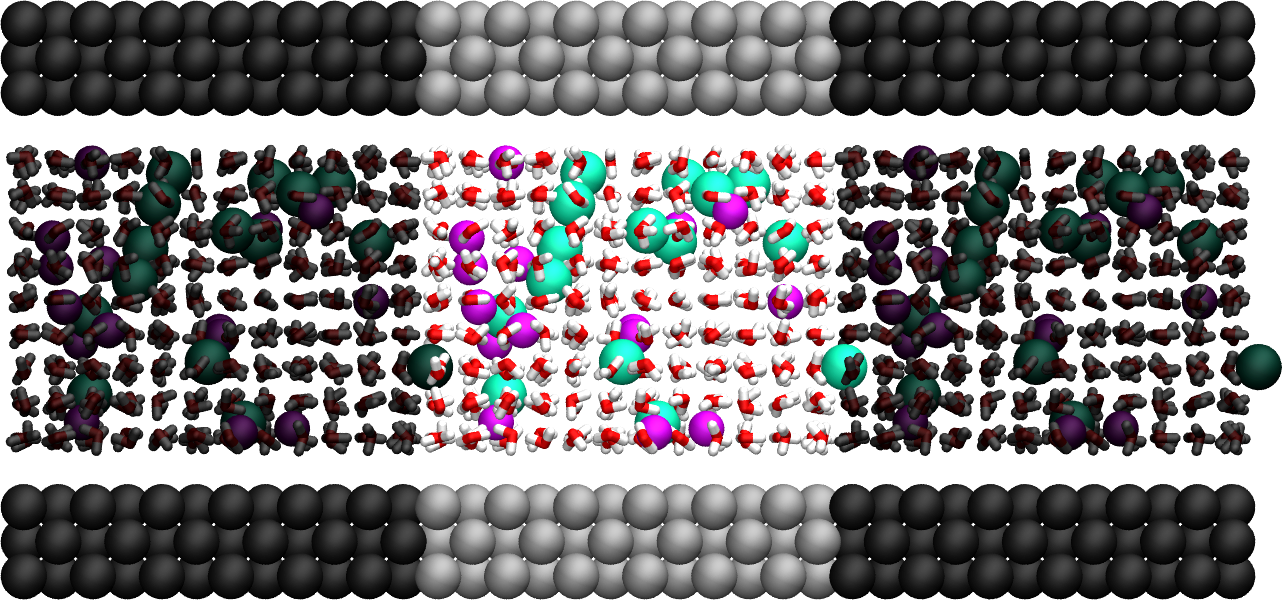

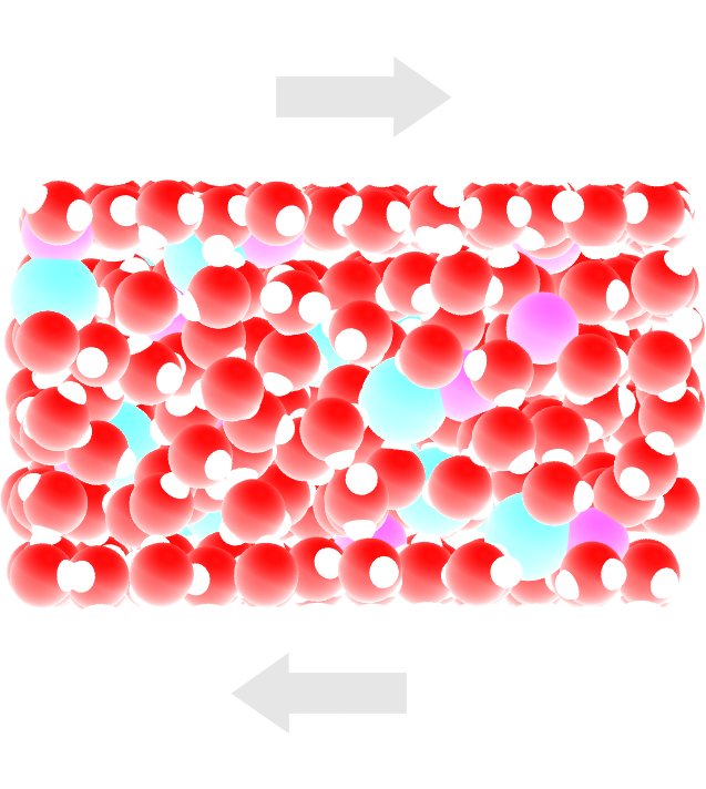
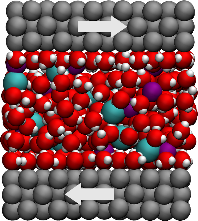
Figure: Side view of the system. Periodic images are represented in darker colors. Water molecules are in red and white, \(\text{Na}^+\) ions in purple, \(\text{Cl}^-\) ions in lime, and wall atoms in gray. Note the absence of atomic defect at the cell boundaries. See the corresponding video.
Always check that your system has been correctly created by looking at the periodic images. Atomic defects may occur at the boundary.
Energy minimization
Why is energy minimization necessary?
It is clear from the way the system has been created that the atoms are not at equilibrium distances from each other. Indeed, some ions added using the create_atoms commands are too close to the water molecules. If we were to start a normal (i.e. with a timestep of about 1 fs) molecular dynamics simulation now, the atoms would exert huge forces on each other, accelerate brutally, and the simulation would likely fail.
Dealing with overlapping atoms
MD simulations failing due to overlapping atoms are extremely common. If it occurs, you can either
delete the overlapping atoms using the delete_atoms command of LAMMPS,
move the atoms to more reasonable distances before the simulation starts using energy minimization, or using molecular dynamics with a small timestep.
Let us move the atoms and place them in more energetically favorable positions before starting the simulation. Let us call this step energy minimization, although it is not a conventional minimization as done for instance in tutorial Lennard-Jones fluid. Instead, a molecular dynamics simulation will be performed here, with some techniques employed to prevent the system from exploding due to overlapping atoms.
To perform this energy minimization, let us create a new folder named minimization/ next to systemcreation/, and create a new input file named input.lammps in it. Copy the following lines in input.lammps:
boundary p p p
units real
atom_style full
bond_style harmonic
angle_style harmonic
pair_style lj/cut/tip4p/long 1 2 1 1 0.1546 12.0
kspace_style pppm/tip4p 1.0e-4
kspace_modify slab 3.0

read_data ../systemcreation/system.data

include ../PARM.lammps
include ../GROUP.lammps
The only difference from the previous input is that instead of creating a new box and new atoms, we open the previously created file system.data located in systemcreation/. The file system.data contains the definition of the simulation box and the positions of the atoms.
Now, let us create a first simulation step using a relatively small timestep (\(0.5\,\text{fs}\)) and a low temperature of \(T = 1\,\text{K}\):
fix mynve fluid nve/limit 0.1
fix myber fluid temp/berendsen 1 1 100
fix myshk H2O shake 1.0e-4 200 0 b 1 a 1
timestep 0.5
Just like fix nve, the fix nve/limit command performs constant NVE integration to update the positions and velocities of the atoms at each timestep. The difference is that fix nve/limit also limits the maximum distance atoms can travel at each timestep. The chosen maximum distance in \(0.1~\text{Å}\). Because the fix nve/limit is applied to the group fluid, only the water molecules and ions will move.
The fix temp/berendsen rescales the velocities of the atoms to force the temperature of the system to reach the desired value of \(1~\text{K}\), and the SHAKE algorithm is used in order to maintain the shape of the water molecules.
Let us also print the atom positions in a .lammpstrj file and control the printing of thermodynamic outputs by adding the following lines to input.lammps:
dump mydmp all atom 1000 dump.lammpstrj
thermo 200
Finally, let us run for 4000 steps. Add the following lines to input.lammps:
run 4000
In order to better equilibrate the system, let us perform two additional steps with a larger timestep and a higher imposed temperature:
fix myber fluid temp/berendsen 300 300 100
timestep 1.0

run 4000

unfix mynve
fix mynve fluid nve

run 4000

write_data system.data nocoeff
For the last of the three steps, fix nve is used instead of nve/limit, which will allow for a better relaxation of the atom positions.
When running the input.lammps file with LAMMPS, you should see that the total energy of the system decreases during the first of the 3 steps, before re-increasing a little after the temperature is increased from 1 to \(300\,\text{K}\).
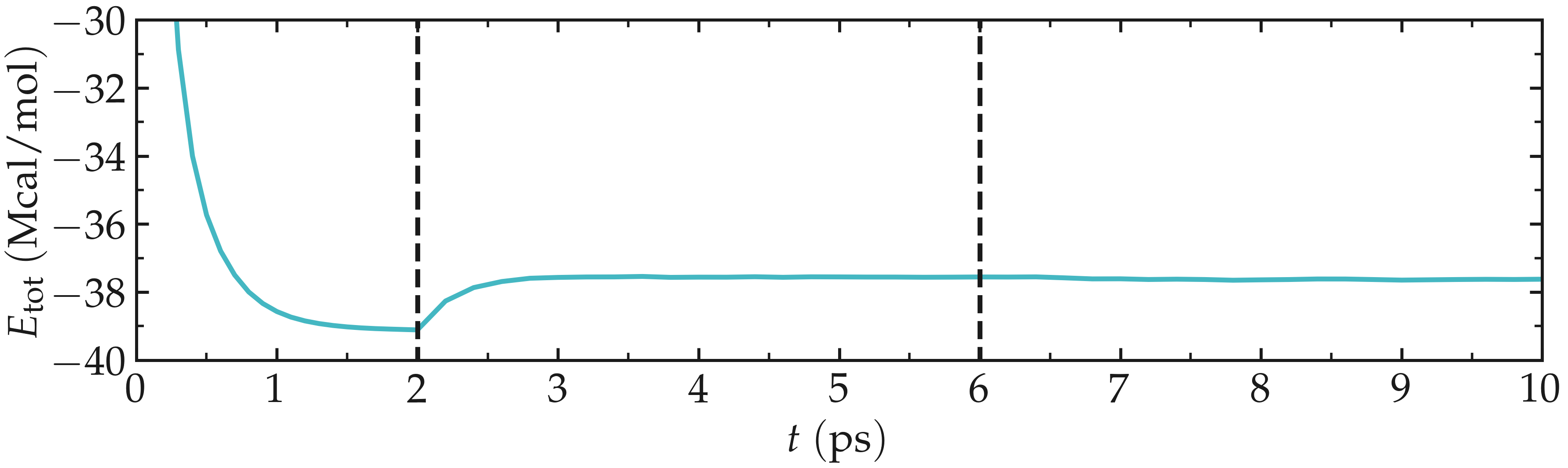
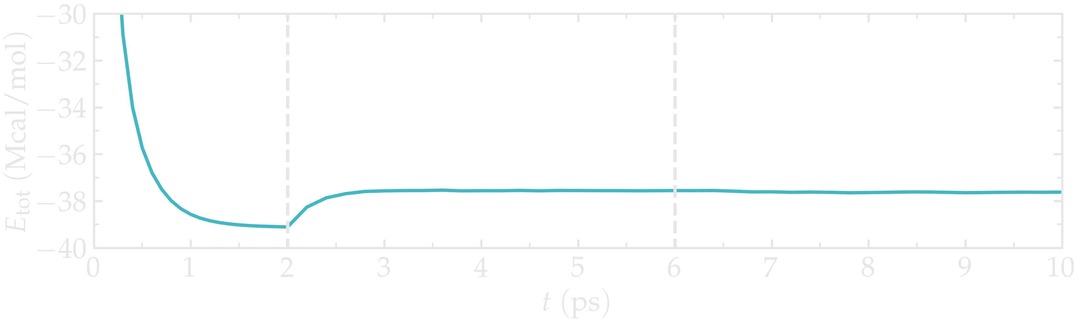
Figure: Total energy of the system \(E_\text{tot}\) as a function of time \(t\) extracted from the log file using Python and lammps_logfile. The vertical dashed lines demarcate the three consecutive steps.
If you look at the trajectory using VMD, you will see that some of the atoms are moving, particularly those that were initially in problematic positions.
System equilibration
Let us equilibrate further the entire system by letting both fluid and piston relax at ambient temperature.
Create a new folder called equilibration/ next to the previously created folders, and create a new input.lammps file in it. Add the following lines to input.lammps:
boundary p p f
units real
atom_style full
bond_style harmonic
angle_style harmonic
pair_style lj/cut/tip4p/long 1 2 1 1 0.1546 12.0
kspace_style pppm/tip4p 1.0e-4
kspace_modify slab 3.0

read_data ../minimization/system.data

include ../PARM.lammps
include ../GROUP.lammps

fix mynve all nve
fix myber all temp/berendsen 300 300 100
fix myshk H2O shake 1.0e-4 200 0 b 1 a 1
fix myrct all recenter NULL NULL 0
timestep 1.0
The fix recenter has no influence on the dynamics, but will keep the system in the center of the box, which makes the visualization easier.
Then, add the following lines to input.lammps for the trajectory visualization and output:
dump mydmp all atom 1000 dump.lammpstrj
thermo 500
variable walltopz equal xcm(walltop,z)
variable wallbotz equal xcm(wallbot,z)
variable deltaz equal v_walltopz-v_wallbotz
fix myat1 all ave/time 100 1 100 v_deltaz file interwall_distance.dat
The first two variables extract the centers of mass of the two walls. Then, the deltaz variable is used to calculate the distance between the two variables walltopz and wallbotz, i.e. the distance between the two walls.
Finally, let us add the run command:
run 30000
write_data system.data nocoeff
Run the input.lammps file using LAMMPS.
As seen from the data printed by fix myat1, the distance between the two walls reduces until it reaches an equilibrium value.
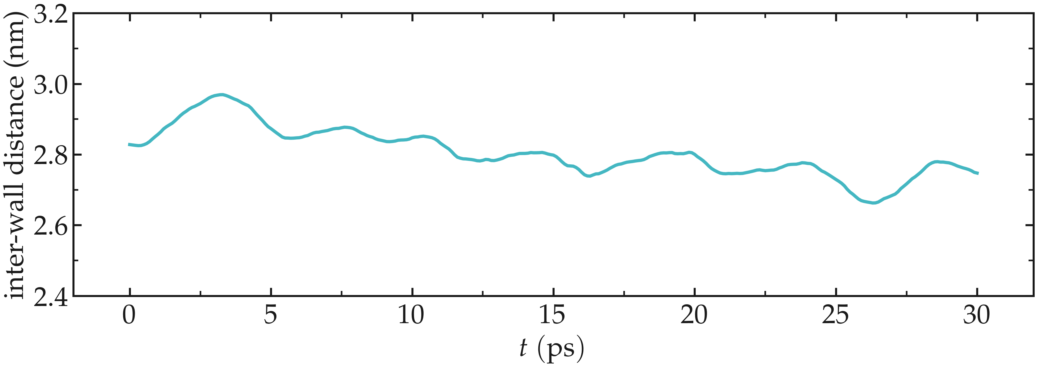
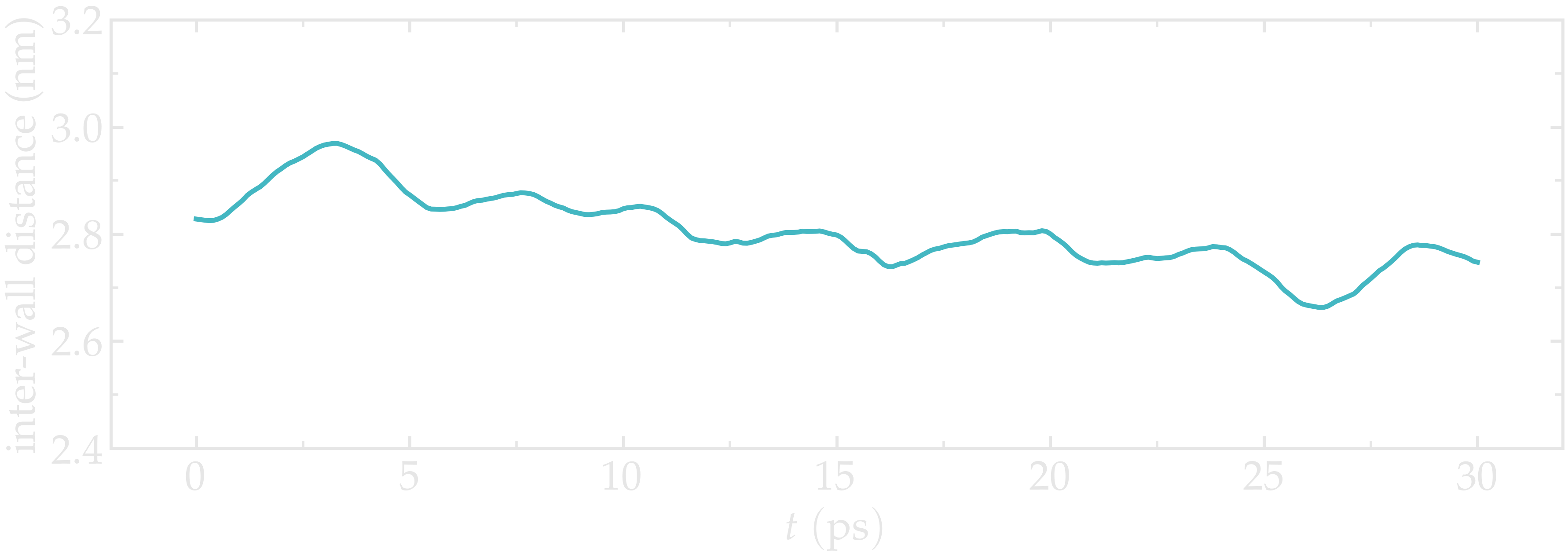
Figure: Distance between the walls as a function of time. After a few picoseconds, the distance between the two walls equilibrates near its final value.
Note that it is generally recommended to run longer equilibration. Here, for instance, the slowest process in the system is probably the ionic diffusion. Therefore, the equilibration should in principle be longer than the time the ions need to diffuse over the size of the pore (\(\approx 1.2\,\text{nm}\)), i.e. on the order of half a nanosecond.
Imposed shearing
From the equilibrated configuration, let us impose a lateral motion to the two walls and shear the electrolyte. In a new folder called shearing/, create a new input.lammps file that starts like the previous ones:
boundary p p f
units real
atom_style full
bond_style harmonic
angle_style harmonic
pair_style lj/cut/tip4p/long 1 2 1 1 0.1546 12.0
kspace_style pppm/tip4p 1.0e-4
kspace_modify slab 3.0
Let us import the previously equilibrated data, include the parameter and group files, and then deal with the dynamics of the system.
read_data ../equilibration/system.data

include ../PARM.lammps
include ../GROUP.lammps

fix mynve all nve
compute Tfluid fluid temp/partial 0 1 1
fix myber1 fluid temp/berendsen 300 300 100
fix_modify myber1 temp Tfluid
compute Twall wall temp/partial 0 1 1
fix myber2 wall temp/berendsen 300 300 100
fix_modify myber2 temp Twall
fix myshk H2O shake 1.0e-4 200 0 b 1 a 1
fix myrct all recenter NULL NULL 0
One difference with the previous input is that, here, two thermostats are used, one for the fluid (myber1) and one for the solid (myber2). The use of fix_modify together with compute temp ensures that the right temperature value is used by the thermostats.
The use of temperature compute with temp/partial 0 1 1 is meant to exclude the x coordinate from the thermalization, which is important since a large velocity will be imposed along x.
Then, let us impose the velocity of the two walls by adding the following commands to input.lammps:
fix mysf1 walltop setforce 0 NULL NULL
fix mysf2 wallbot setforce 0 NULL NULL
velocity wallbot set -2e-4 NULL NULL
velocity walltop set 2e-4 NULL NULL
The setforce commands cancel the forces on walltop and wallbot, respectively. Therefore the atoms of the two groups do not experience any force from the rest of the system. In the absence of force acting on those atoms, they will conserve their initial velocity.
The velocity commands act only once and impose the velocity of the atoms of the groups wallbot and walltop, respectively.
Finally, let us dump the atom positions, extract the velocity profiles using several ave/chunk commands, extract the force applied on the walls, and then run for \(200\,\text{ps}\) Add the following lines to input.lammps:
dump mydmp all atom 5000 dump.lammpstrj
thermo 500
thermo_modify temp Tfluid

compute cc1 H2O chunk/atom bin/1d z 0.0 1.0
compute cc2 wall chunk/atom bin/1d z 0.0 1.0
compute cc3 ions chunk/atom bin/1d z 0.0 1.0

fix myac1 H2O ave/chunk 10 15000 200000 &
cc1 density/mass vx file water.profile_1A.dat
fix myac2 wall ave/chunk 10 15000 200000 &
cc2 density/mass vx file wall.profile_1A.dat
fix myac3 ions ave/chunk 10 15000 200000 &
cc3 density/mass vx file ions.profile_1A.dat

fix myat1 all ave/time 10 100 1000 f_mysf1[1] f_mysf2[1] file forces.dat

timestep 1.0
run 200000
write_data system.data nocoeff
Here, a binning of \(1\,\text{Å}\) is used for the density profiles generated by the ave/chunk commands. For smoother profiles, you can reduce its value.
The averaged velocity profile of the fluid can be plotted. As expected for such Couette flow geometry, the velocity of the fluid is found to increase linearly along \(z\).
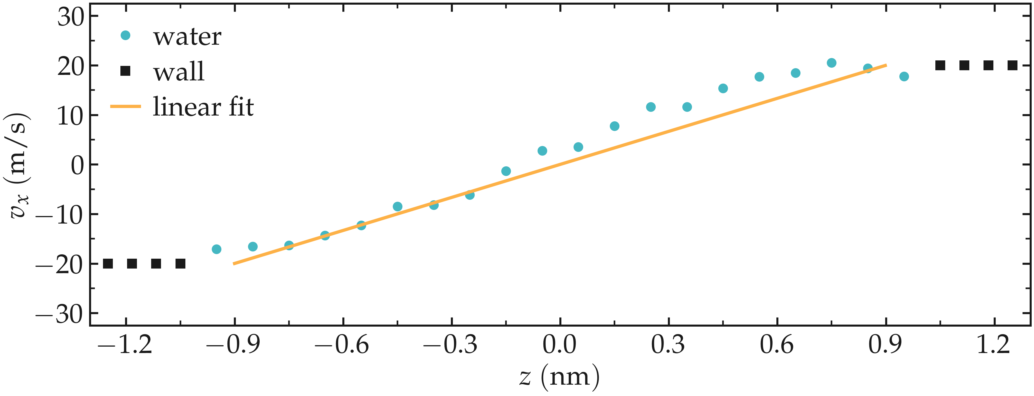
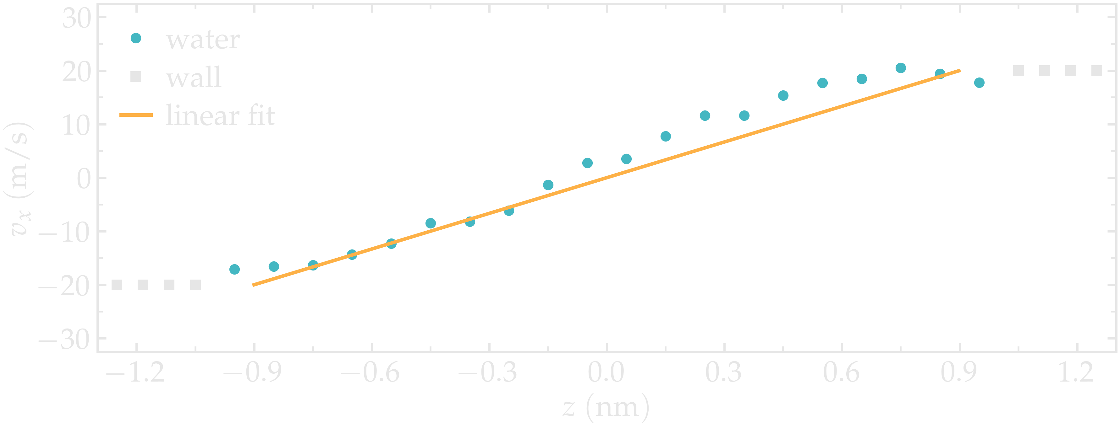
Figure: Velocity profiles for water molecules, ions and walls along the z axis. The line is a linear fit assuming that the pore size is \(h = 1.8\,\text{nm}\).
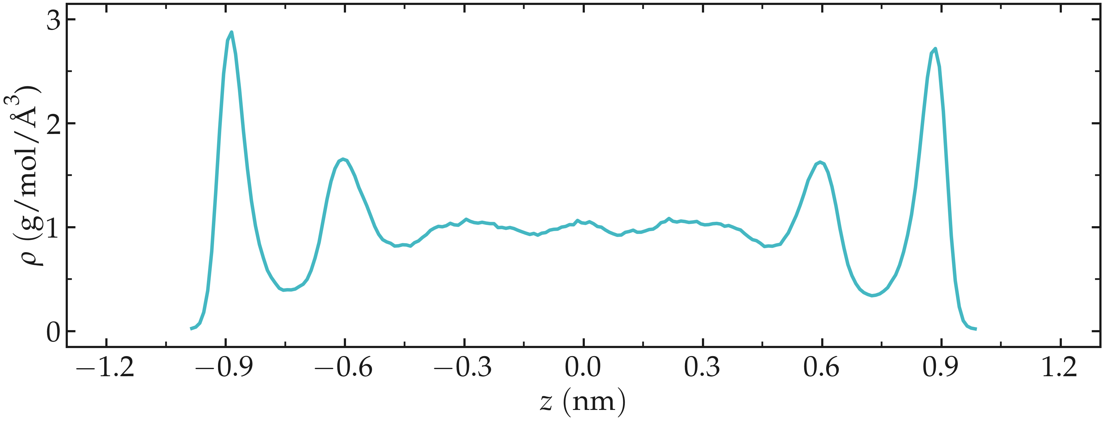
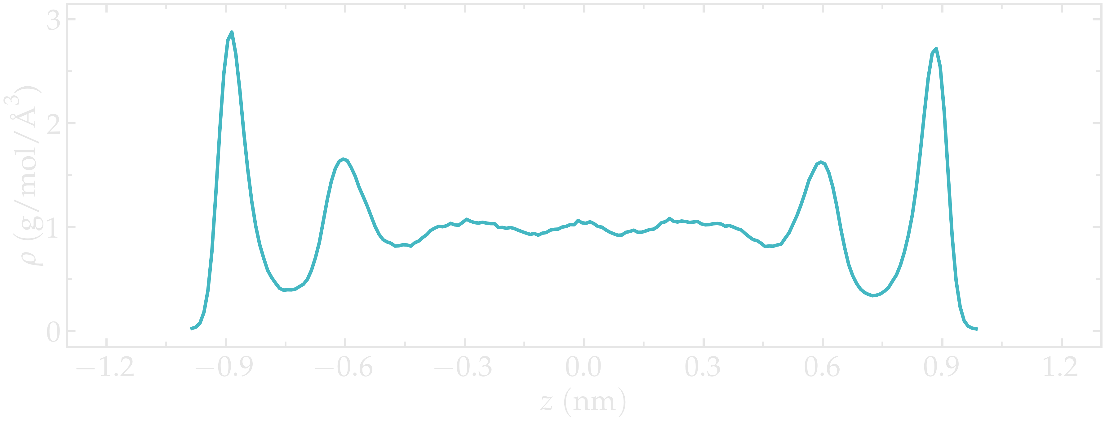
Figure: Water density \(\rho\) profile along the z axis.
From the force applied by the fluid on the solid, one can extract the stress within the fluid, which allows for the measurement of its viscosity \(\dot{\eta}\) according to gravelle2021: \(\eta = \tau / \dot{\gamma}\) where \(\tau\) is the stress applied by the fluid on the shearing wall, and \(\dot{\gamma}\) the shear rate (which is imposed here) [40]. Here, the shear rate is approximatively \(\dot{\gamma} = 16 \cdot 10^9\,\text{s}^{-1}\), and using a surface area of \(A = 6 \cdot 10^{-18}\,\text{m}^2\), one gets an estimate for the shear viscosity for the confined fluid of \(\eta = 6.6\,\text{mPa.s}\).
The viscosity calculated at such a high shear rate may differ from the expected bulk value. In general, it is recommended to use a lower value for the shear rate. Note that for lower shear rates, the ratio of noise-to-signal is larger, and longer simulations are needed.
Another important point to keep in mind is that the viscosity of a fluid next to a solid surface is typically larger than in bulk due to interaction with the walls [41]. Therefore, one expects the present simulation to return a viscosity that is slightly larger than what would be measured in the absence of a wall.
You can access the input scripts and data files that are used in these tutorials from this Github repository. This repository also contains the full solutions to the exercises.
Going further with exercises
Each exercise comes with a proposed solution, see Solutions to the exercises.
Induce a Poiseuille flow
Instead of inducing a shearing of the fluid using the walls, induce a net flux of the liquid in the direction tangential to the walls. The walls must be kept immobile.
Extract the velocity profile, and make sure that the resulting velocity profile is consistent with the Poiseuille equation, which can be derived from the Stokes equation \(\eta \nabla \textbf{v} = - \textbf{f} \rho\) where \(f\) is the applied force, \(\rho\) is the fluid density, \(\eta\) is the fluid viscosity.
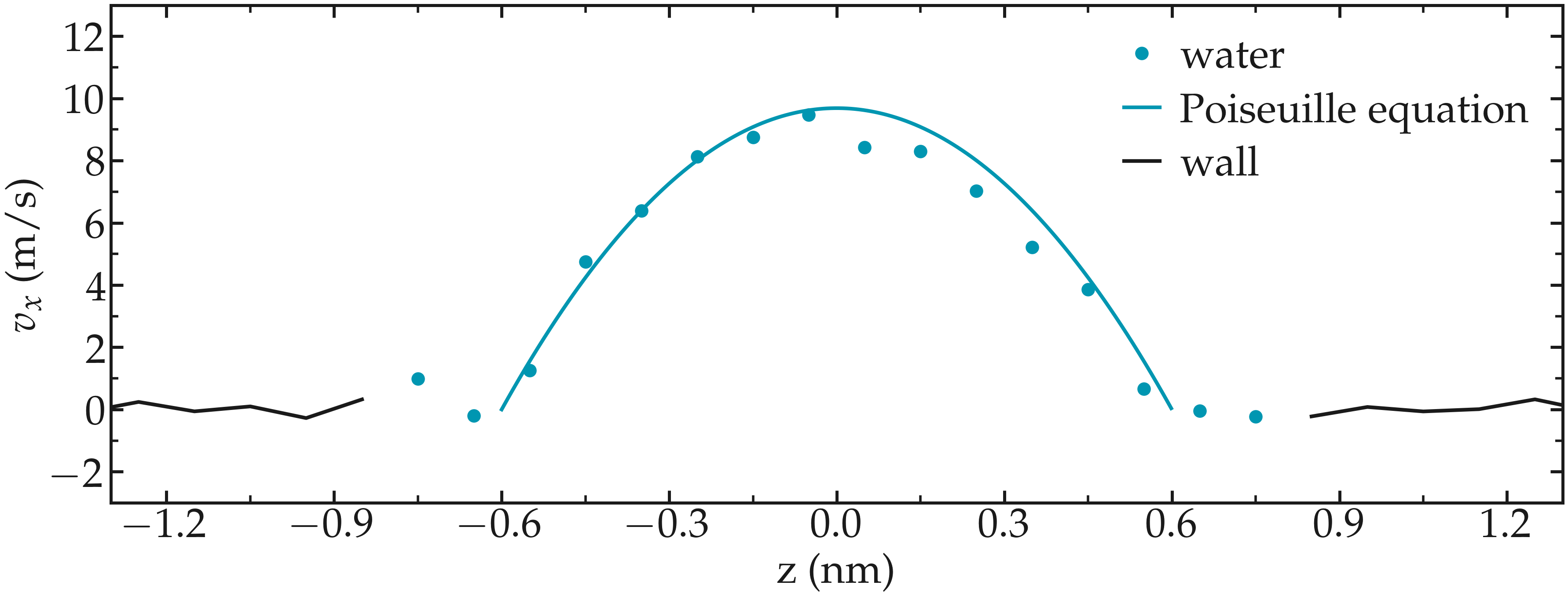
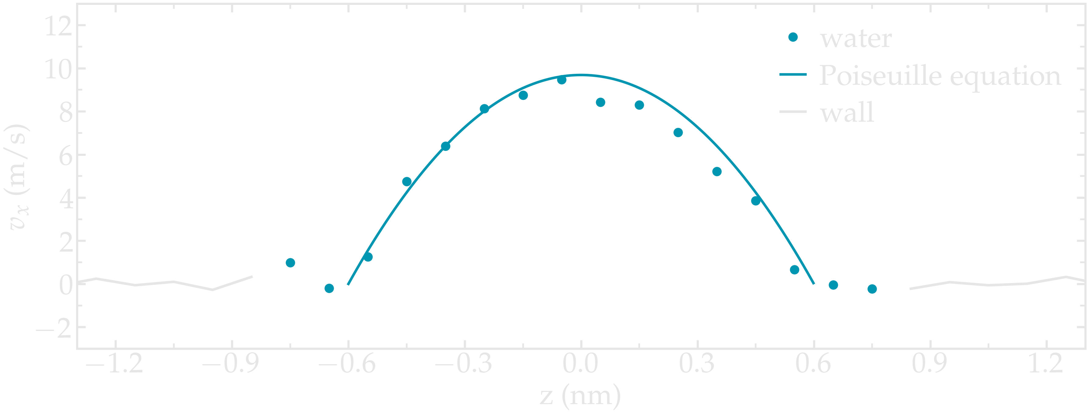
Figure: Velocity profiles of the water molecules along the z axis (disks). The line is the Poiseuille equation.
An important step is to choose the proper value for the additional force.