Water adsorption in silica

Dealing with a varying number of molecules

The objective of this tutorial is to combine molecular dynamics and grand canonical Monte Carlo simulations to compute the adsorption of water molecules in a cracked silica material.

This tutorial illustrates the use of the grand canonical ensemble in molecular simulation, an open ensemble in which the number of atoms within the simulation box is not constant. When using the grand canonical ensemble, it is possible to impose the chemical potential (or pressure, or fugacity) of a given fluid in a nanoporous structure.

If you are completely new to LAMMPS, I recommend that you follow this tutorial on a simple Lennard-Jones fluid first.

Looking for support in molecular simulations?

I provide assistance for LAMMPS projects. See the Contact me page.

This tutorial is compatible with the 2Aug2023 LAMMPS version.

Generation of the silica block

Let us first generate a block of amorphous silica (SiO2). To do so, we are going to replicate a building block containing 3 Si and 6 O atoms.

Create two folders side by side, and name them respectively Potential/ and SilicaBlock/.

An initial data file for the SiO atoms can be downloaded by clicking here. Save it in SilicaBlock/. This data file contains the coordinates of the 9 atoms, their masses, and their charges. The .data file can be directly read by LAMMPS using the read_data command. Let us replicate these atoms using LAMMPS, and apply an annealing procedure to obtain a block of amorphous silica.

About annealing procedure

The annealing procedure consists of adjusting the system temperature in successive steps. Here, a large initial temperature is chosen to ensure the melting of the SiO2 structure. Then, several steps are used to progressively cool down the system until it solidifies and forms amorphous silica. Depending on the material, different cooling velocities can sometimes lead to different crystal structures or different degrees of defect.

Vashishta potential

Create a new input file named input.lammps in the SilicaBlock/ folder, and copy the following lines in it:

units metal
boundary p p p
atom_style full
pair_style vashishta
neighbor 1.0 bin
neigh_modify delay 1

The main difference with some of the previous tutorials is the use of the Vashishta pair style. Download the Vashishta potential by clicking here, and copy it within the Potential/ folder.

About the Vashishta potential

The Vashishta potential is a bond-angle energy-based potential, it deduces the bonds between atoms from their relative positions [33]. Therefore, there is no need to provide the bond and angle information as we do with classic force fields like GROMOS or AMBER. When used with LAMMPS, the Vashishta potential requires the use of the metal units system. Bond-angle energy-based potentials are more computationally heavy than classical force fields and require the use of a smaller timestep, but they allow for the modeling of bond formation and breaking, which is what we need here as we want to create a crack in the silica.

Let us then import the system made of 9 atoms, and replicate it four times in all three directions of space, thus creating a system with 576 atoms. Add the following lines to input.lammps:

read_data SiO.data
replicate 4 4 4

Then, let us specify the pair coefficients by indicating that the first atom type is Si, and the second is O. Let us also add a dump command for printing out the positions of the atoms every 5000 steps:

pair_coeff * * ../Potential/SiO.1990.vashishta Si O

Let us add some commands to input.lammps to help us follow the evolution of the system, such as its temperature, volume, and potential energy:

dump dmp all atom 5000 dump.lammpstrj
variable myvol equal vol
variable mylx equal lx
variable myly equal ly
variable mylz equal lz
variable mypot equal pe
variable mytemp equal temp
fix myat1 all ave/time 10 100 1000 v_mytemp file temperature.dat
fix myat2 all ave/time 10 100 1000 &
v_myvol v_mylx v_myly v_mylz file dimensions.dat
fix myat3 all ave/time 10 100 1000 v_mypot file potential-energy.dat
thermo 1000

Annealing procedure

Finally, let us create the last part of our script. The annealing procedure is made of four consecutive runs. First, a \(50\,\text{ps}\) phase at \(T = 6000\,\text{K}\) and isotropic pressure coupling with desired pressure \(p = 100\,\text{atm}\):

velocity all create 6000 4928459 rot yes dist gaussian
fix npt1 all npt temp 6000 6000 0.1 iso 100 100 1
timestep 0.001
run 50000

Then, a second phase during which the system is cooled down from \(T = 6000\,\text{K}\) to \(T = 4000\,\text{K}\). An anisotropic pressure coupling is used, allowing all three dimensions of the box to evolve independently from one another:

fix npt1 all npt temp 6000 4000 0.1 aniso 100 100 1
run 50000

Then, let us cool down the system further while also reducing the pressure, then perform a small equilibration step at the final desired condition, \(T = 300\,\text{K}\) and \(p = 1\,\text{atm}\).

fix npt1 all npt temp 4000 300 0.1 aniso 100 1 1
run 200000
fix npt1 all npt temp 300 300 0.1 aniso 1 1 1
run 50000

write_data amorphousSiO.data

Disclaimer – I created this procedure by intuition and not from proper calibration, do not copy it without making your tests if you intend to publish your results.

Anisotropic versus isotropic barostat

Here, an isotropic barostat is used for the melted phase at \(T = 6000\,\text{K}\), and then an anisotropic barostat is used for all following phases. With the anisotropic barostat, all three directions of space are adjusted independently from one another. Such anisotropic barostat is usually a better choice for a solid phase. For a liquid or a gas, the isotropic barostat is usually the best choice.

The simulation takes about 15-20 minutes on 4 CPU cores.

Let us check the evolution of the temperature from the temperature.dat file. Apart from an initial spike (which may be due to an initial bad configuration, probably harmless here), the temperature follows well the desired annealing procedure.

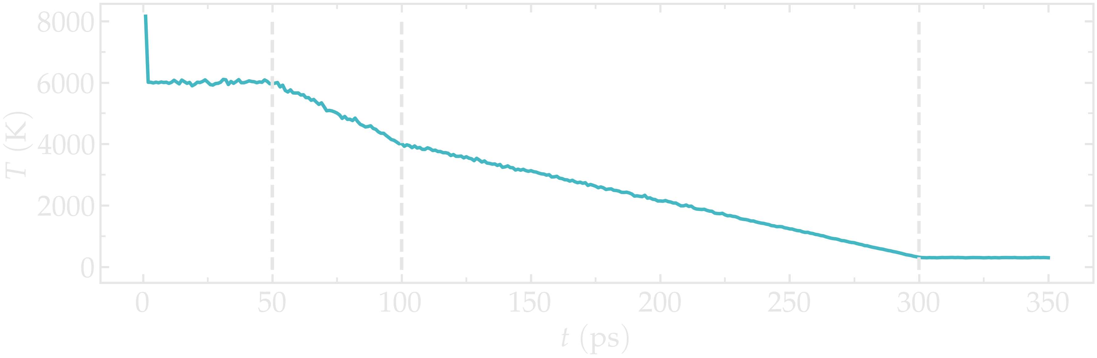
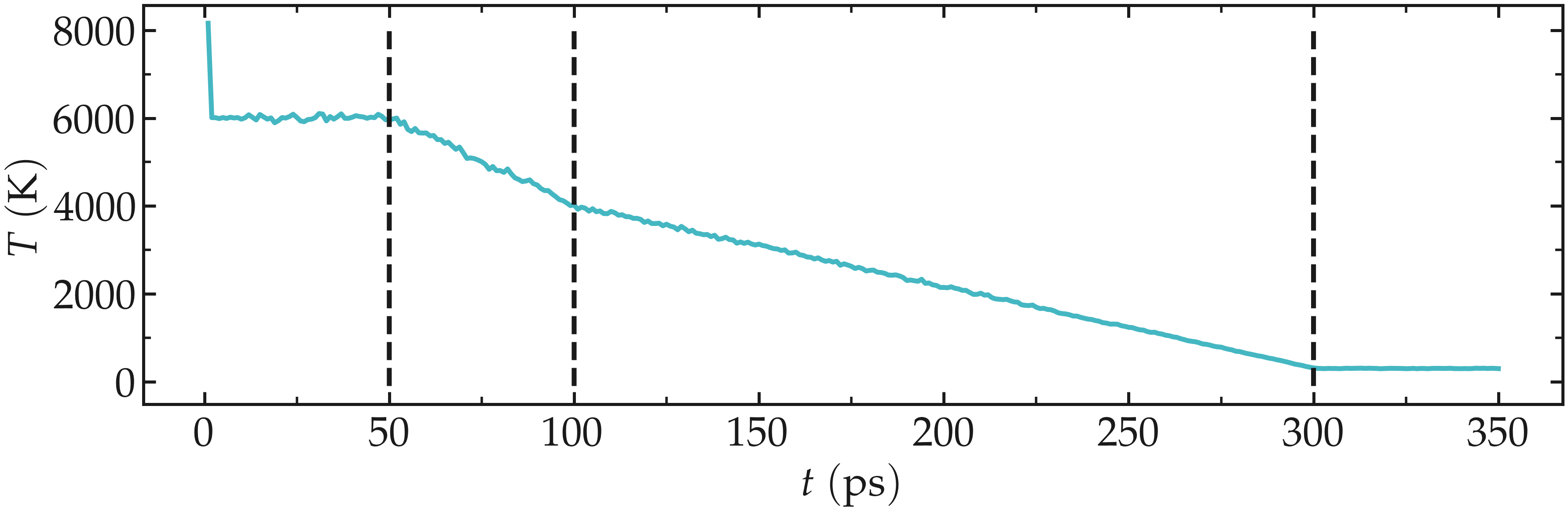
Figure: Temperature of the system during annealing. The vertical dashed lines mark the transition between the different phases of the simulations.

Let us also make sure that the box was indeed deformed isotropically during the first stage of the simulation, and then anisotropically by plotting the evolution of the box dimensions over time.

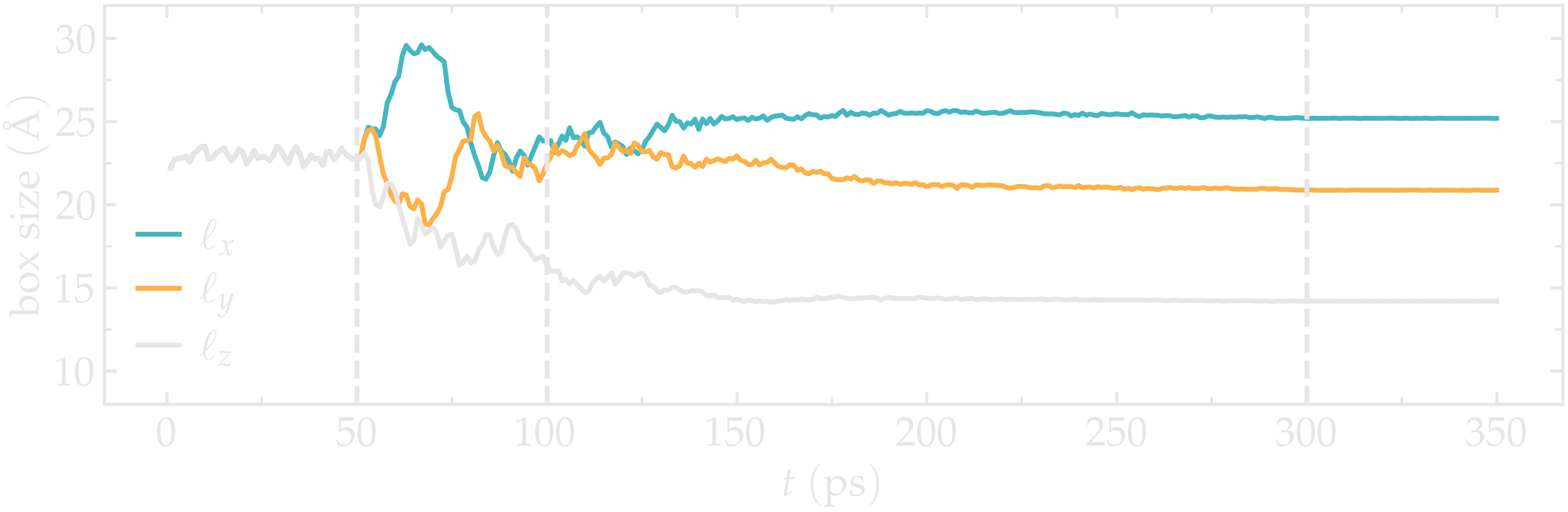
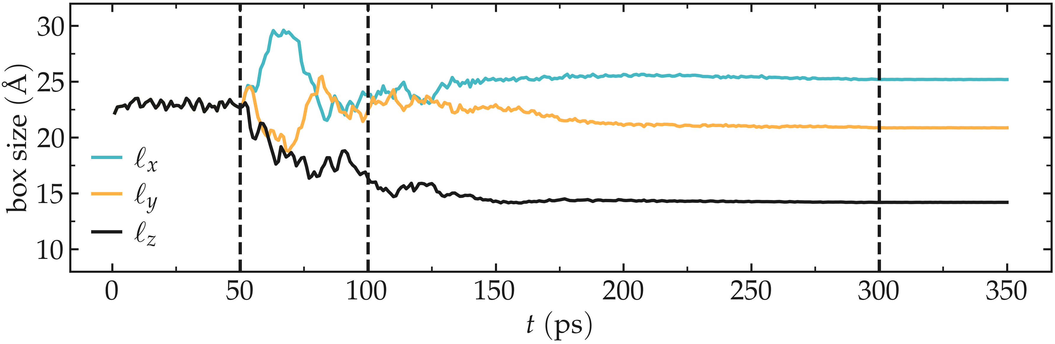
Figure: Box dimensions during annealing. The vertical dashed lines mark the transition between the different phases of the simulations.

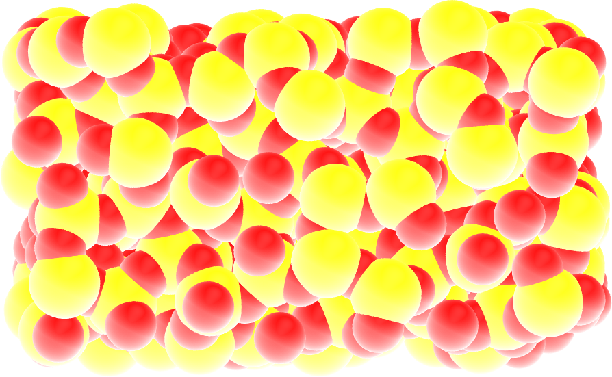
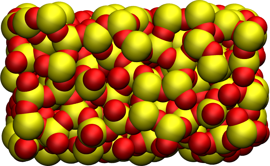
Figure: Snapshot of the final amorphous silica (SiO2) with Si atom in yellow and O atoms in red.

After running the simulation, the final LAMMPS topology file named amorphousSiO.data will be located in SilicaBlock/. Alternatively, if you are only interested in the next steps of this tutorial, you can download it by clicking here.

Tip for research project

In the case of a research project, the validity of the generated structure must be tested and compared to reference values, ideally from experiments. For instance, radial distribution functions or Young modulus can both be compared to experimental values. This is beyond the scope of this tutorial.

Cracking the silica

Let us dilate the block of silica to create a crack. Create a new folder called Cracking/ next to SilicaBlock/, and create a new input.lammps file starting with familiar lines:

units metal
boundary p p p
atom_style full
neighbor 1.0 bin
neigh_modify delay 1

read_data ../SilicaBlock/amorphousSiO.data

pair_style vashishta
pair_coeff * * ../Potential/SiO.1990.vashishta Si O
dump dmp all atom 1000 dump.lammpstrj

Then, let us progressively increase the size of the box in the z-direction, thus forcing the silica to deform and eventually crack. To do so, let us make a loop using the jump command. At every step of the loop, the box dimension over x will be multiplied by a factor 1.005. Here, we use a NVT thermostat because we want to impose a deformation of the volume.

On using barostat during deformation

Here, box deformations are applied in the x-direction, while the y and z box dimensions are kept constants.

Another possible choice would be to apply a barostat along the y and z direction, allowing the system more freedom to deform. In LAMMPS, this can be done by using :

fix npt1 all npt temp 300 300 0.1 y 1 1 1 z 1 1 1

instead of:

fix nvt1 all nvt temp 300 300 0.1

Here, the second option will be used.

Add the following lines to the input.lammps:

fix nvt1 all nvt temp 300 300 0.1
timestep 0.001
thermo 1000
variable var loop 45
label loop
change_box all x scale 1.005 remap
run 2000
next var
jump input.lammps loop
run 20000
write_data dilatedSiO.data

You can use different scale factor (here 1.005) or different number of steps in the loop (here 45) if you want to generate different defects in the silica.

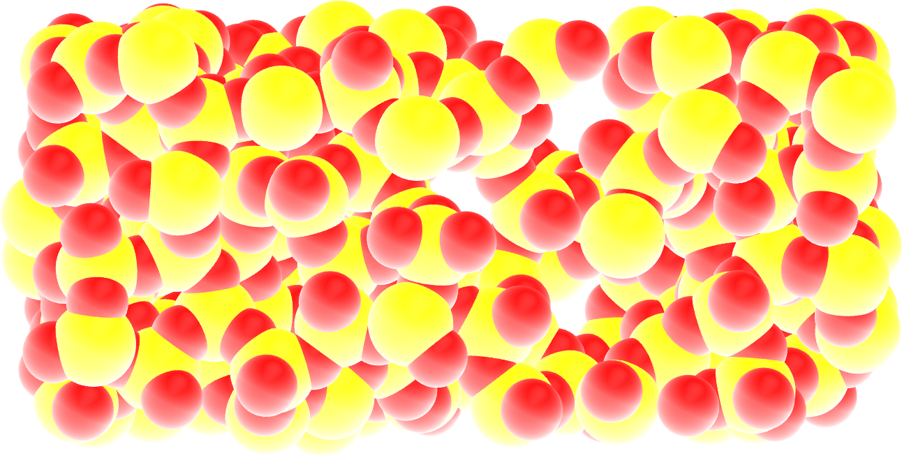
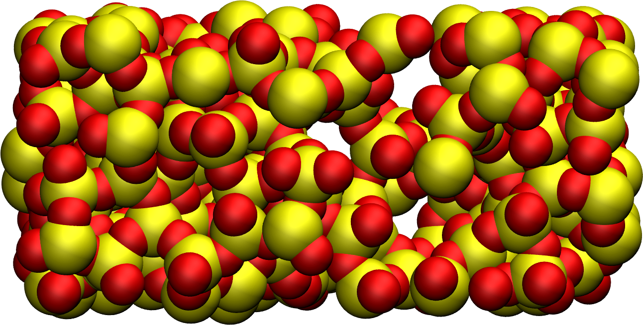
Figure: Block of silica after deformation, with some visible holes.

After the dilatation, a final equilibration step of duration 20 picoseconds is performed. If you look at the dump.lammpstrj file using VMD, you can see the dilatation occurring step-by-step, and the atoms progressively adjusting to the box dimensions.

At first, the deformations are reversible (elastic regime). At some point, bonds start breaking and dislocations appear (plastic regime).

Alternatively, you can download the final state directly by clicking here. The final system with the crack resembles:

Passivated silica

In ambient conditions, Some of the surface SiO2 atoms are chemically passivated by forming covalent bonds with hydrogen (H) atoms. For the sake of simplicity, we are not going to add surface hydrogen atoms here. An example of a procedure allowing for properly inserting hydrogen atoms is given as an exercise from Reactive silicon dioxide.

Adding water

In order to add the water molecules to the silica, we are going to use the Monte Carlo method in the grand canonical ensemble (GCMC). In short, the system is put into contact with a virtual reservoir of a given chemical potential \(\mu\), and multiple attempts to insert water molecules at random positions are made. Attempts are either accepted or rejected based on energy considerations.

Using hydrid potentials

Create a new folder called Addingwater/. Download and save the template file for the water molecule within Addingwater/.

Create a new input file called input.lammps within Addingwater/, and copy the following lines into it:

units metal
boundary p p p
atom_style full
neighbor 1.0 bin
neigh_modify delay 1
pair_style hybrid/overlay vashishta lj/cut/tip4p/long 3 4 1 1 0.1546 10
kspace_style pppm/tip4p 1.0e-4
bond_style harmonic
angle_style harmonic

There are several differences with the previous input files used in this tutorial. From now on, the system will combine water and silica, and therefore two force fields are combined: Vashishta for SiO, and lj/cut/tip4p/long for TIP4P water model (here the TIP4P/2005 model is used [28]). Combining the two force fields is done using the hybrid/overlay pair style.

About hybrid and hybrid/overlay pair style

From the LAMMPS documentation: The hybrid and hybrid/overlay styles enable the use of multiple pair styles in one simulation. With the hybrid style, exactly one pair style is assigned to each pair of atom types. With the hybrid/overlay and hybrid/scaled styles, one or more pair styles can be assigned to each pair of atom types.

The kspace solver is used to calculate the long range Coulomb interactions associated with tip4p/long. Finally, the style for the bonds and angles of the water molecules are defined, although they are not important since it is a rigid water model.

Before going further, we also need to make a few changes to our data file. Currently, dilatedSiO.data only includes two atom types, but we need four. Copy the previously generated dilatedSiO.data file within Addingwater/. Currently, dilatedSiO.data starts with:

576 atoms
2 atom types

-5.512084438507452 26.09766215010596 xlo xhi
-0.12771230207837192 20.71329001367807 ylo yhi
3.211752393088563 17.373825318513106 zlo zhi

Masses

1 28.0855
2 15.9994

Atoms # full

(...)

Make the following changes to allow for the addition of water molecules. Modify the file so that it looks like the following (with 4 atom types, 1 bond type, 1 angle type, and four masses):

576 atoms
4 atom types
1 bond types
1 angle types

2 extra bond per atom
1 extra angle per atom
2 extra special per atom

0.910777522101565 19.67480018949893 xlo xhi
2.1092682236518137 18.476309487947546 ylo yhi
-4.1701120819606885 24.75568979356097 zlo zhi

Masses

1 28.0855
2 15.9994
3 15.9994
4 1.008

Atoms # full

(...)

Doing so, we anticipate that there will be 4 atom types in the simulations, with O and H of H2O having indexes 3 and 4, respectively. There will also be 1 bond type and 1 angle type. The extra bond, extra angle, and extra special lines are here for memory allocation.

We can continue to fill in the input.lammps file, by adding the system definition:

read_data dilatedSiO.data
molecule h2omol H2O.mol
lattice sc 3
create_atoms 0 box mol h2omol 45585
lattice none 1

group SiO type 1 2
group H2O type 3 4

After reading the data file and defining the h2omol molecule from the txt file, the create_atoms command is used to include some water molecules in the system on a simple cubic lattice. Not adding a molecule before starting the GCMC steps usually lead to failure. Note that here, most water molecules overlap with the silica. These overlapping water molecules will be deleted before starting the simulation.

Then, add the following settings to input.lammps:

pair_coeff * * vashishta ../Potential/SiO.1990.vashishta Si O NULL NULL
pair_coeff * * lj/cut/tip4p/long 0 0
# epsilonSi = 0.00403, sigmaSi = 3.69
# epsilonO = 0.0023, sigmaO = 3.091
pair_coeff 1 3 lj/cut/tip4p/long 0.0057 4.42
pair_coeff 2 3 lj/cut/tip4p/long 0.0043 3.12
pair_coeff 3 3 lj/cut/tip4p/long 0.008 3.1589
pair_coeff 4 4 lj/cut/tip4p/long 0.0 0.0
bond_coeff 1 0 0.9572
angle_coeff 1 0 104.52

variable oxygen atom "type==3"
group oxygen dynamic all var oxygen
variable nO equal count(oxygen)
fix myat1 all ave/time 100 10 1000 v_nO file numbermolecule.dat

fix shak H2O shake 1.0e-4 200 0 b 1 a 1 mol h2omol

The force field Vashishta applies only to Si (type 1) and O of SiO2 (type 2), and not to the O and H of H2O, thanks to the NULL parameters used for atoms of types 3 and 4.

Pair coefficients for lj/cut/tip4p/long are defined between O atoms, as well as between O(SiO)-O(H2O) and Si(SiO)-O(H2O). Therefore, the fluid-solid interactions will be set by Lennard-Jones and Coulomb potentials.

The number of oxygen atoms from water molecules (i.e. the number of molecules) will be printed in the file numbermolecule.dat.

The shake algorithm is used to maintain the shape of the water molecules over time. Some of these features have been seen in previous tutorials.

Let us delete the overlapping water molecules, and print the positions of the remaining atoms in a .lammpstrj file by adding the following lines to input.lammps:

delete_atoms overlap 2 H2O SiO mol yes
dump dmp all atom 1000 dump.init.lammpstrj

GCMC simulation

To prepare for the GCMC simulation, let us make the first equilibration step by adding the following lines to input.lammps:

compute_modify thermo_temp dynamic yes
compute ctH2O H2O temp
compute_modify ctH2O dynamic yes
fix mynvt1 H2O nvt temp 300 300 0.1
fix_modify mynvt1 temp ctH2O
compute ctSiO SiO temp
fix mynvt2 SiO nvt temp 300 300 0.1
fix_modify mynvt2 temp ctSiO
timestep 0.001
thermo 1000
run 5000

On thermostating groups instead of the entire system

Two different thermostats are used for SiO and for H2O, respectively. Using separate thermostats are usually better when the system contains two separate species, such as a solid and a liquid. It is particularly important to use two thermostats here because the number of water molecules will fluctuate with time.

The compute_modify with dynamic yes for water is used to specify that the number of molecules is not constant.

Finally, let us use the fix gcmc and perform the grand canonical Monte Carlo steps. Add the following lines into input.lammps:

variable tfac equal 5.0/3.0
variable xlo equal xlo+0.1
variable xhi equal xhi-0.1
variable ylo equal ylo+0.1
variable yhi equal yhi-0.1
variable zlo equal zlo+0.1
variable zhi equal zhi-0.1
region system block ${xlo} ${xhi} ${ylo} ${yhi} ${zlo} ${zhi}
fix fgcmc H2O gcmc 100 100 0 0 65899 300 -0.5 0.1 &
    mol h2omol tfac_insert ${tfac} group H2O shake shak &
    full_energy pressure 10000 region system
run 45000
write_data SiOwithwater.data
write_dump all atom dump.lammpstrj

Dirty fix

The region system was created to avoid the error Fix gcmc region extends outside simulation box which seems to occur with the 2Aug2023 LAMMPS version.

The tfac_insert option ensures that the correct estimate is made for the temperature of the inserted water molecules by taking into account the internal degrees of freedom. Running this simulation, you should see the number of molecules increasing progressively. When using the pressure argument, LAMMPS ignores the value of the chemical potential [here \(\mu = -0.5\,\text{eV}\) which corresponds roughly to ambient conditions (i.e. \(\text{RH} \approx 50\,\%\)).] The large pressure value of 10000 bars was chosen to ensure that some successful insertions of molecules would occur during the extremely short duration of this simulation.

When you run the simulation, make sure that some water molecules remain in the system after the delete_atoms command. You can control that either using the log file or using the numbermolecule.dat data file.

You can see, by looking at the log file, that 280 molecules were added by the create_atoms command (the exact number you get may differ):

Created 840 atoms

You can also see that 258 molecules were immediately deleted, leaving 24 water molecules (the exact number you get may differ):

Deleted 774 atoms, new total = 642
Deleted 516 bonds, new total = 44
Deleted 258 angles, new total = 22

After just a few GCMC steps, the number of molecules starts increasing. Once the crack is filled with water molecules, the number of molecules reaches a plateau.

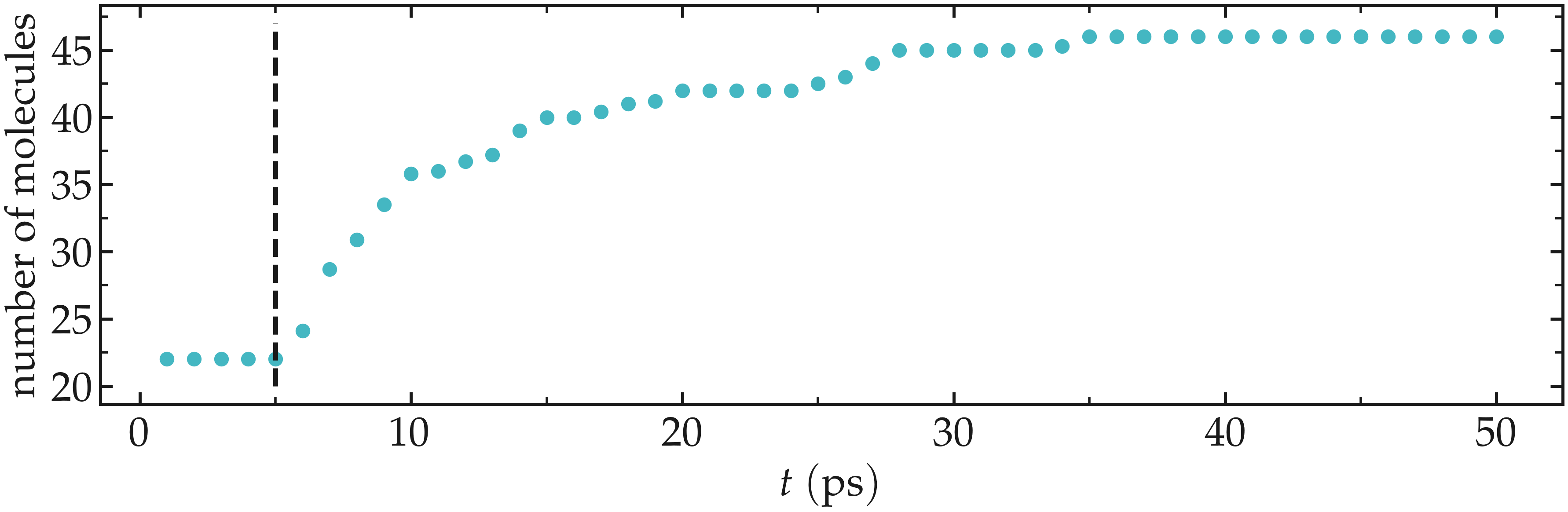
Figure: Number of molecules as a function of time. The dashed vertical line marks the beginning of the GCMC step.

The final number of molecules depends on the imposed pressure, temperature, and on the interaction between water and silica (i.e. its hydrophilicity).

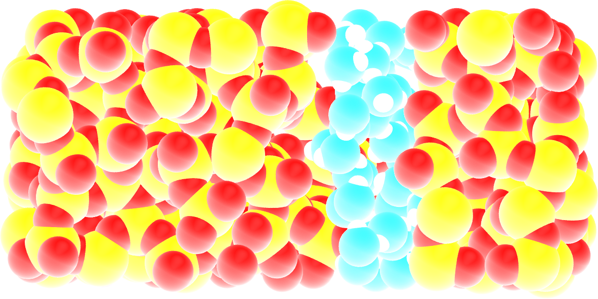
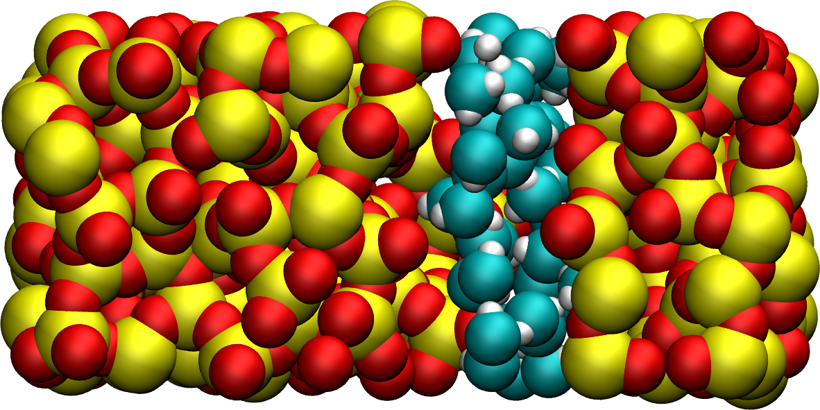
Figure: Snapshot of the silica system after the adsorption of the water molecules, with the oxygen of the water molecules represented in cyan.

Note that GCMC simulations of such dense phases are usually slow to converge due to the very low probability of successfully inserting a molecule. Here, the short simulation duration was made possible by the use of a large pressure.

Vizualising varying number of molecules

By default, VMD fails to properly render systems with varying numbers of atoms.

You can access the input scripts and data files that are used in these tutorials from this Github repository. This repository also contains the full solutions to the exercises.

Going further with exercises

Each comes with a proposed solution, see Solutions to the exercises.

Mixture adsorption

Adapt the existing script and insert both \(\text{CO}_2\) molecules and water molecules within the silica crack using GCMC. Download the CO2 template. The parameters for the \(\text{CO}_2\) molecule are the following:

pair_coeff 5 5 lj/cut/tip4p/long 0.0179 2.625854
pair_coeff 6 6 lj/cut/tip4p/long 0.0106 2.8114421
bond_coeff 2 46.121 1.17
angle_coeff 2 2.0918 180

The atom of type 5 is an oxygen of mass 15.9994, and the atom of type 6 is a carbon of mass 12.011.

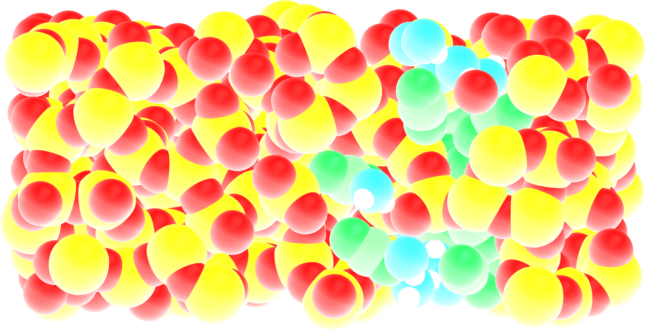
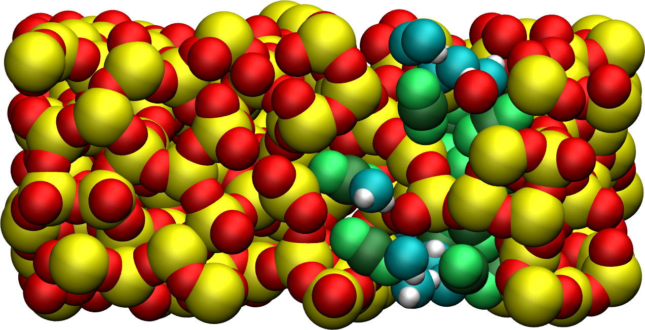
Figure: Cracked silica with adsorbed water and \(\text{CO}_2\) molecules (in green).

Adsorb water in ZIF-8 nanopores

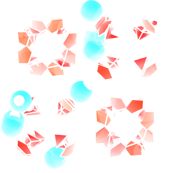
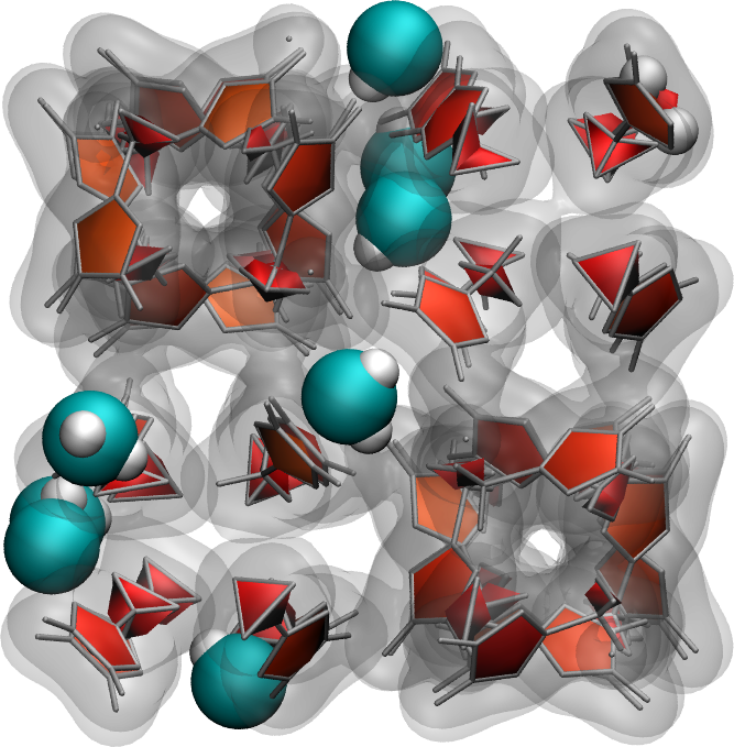
Use the same protocol as the one implemented in this tutorial to add water molecules to a Zif-8 nanoporous material. A snapshot of the system with a few water molecules is shown on the right.

Download the initial Zif-8 structure, the parameters file, and this new water template. The ZIF-8 structure is made of 7 atom types (C1, C2, C3, H2, H3, N, Zn), connected by bonds, angles, dihedrals, and impropers. It uses the same pair_style as water, so there is no need to use hybrid pair_style. Your input file should start like this:

units real
atom_style full
boundary p p p
bond_style harmonic
angle_style harmonic
dihedral_style charmm
improper_style harmonic

pair_style lj/cut/tip4p/long 1 2 1 1 0.105 14.0
kspace_style pppm/tip4p 1.0e-5

special_bonds lj 0.0 0.0 0.5 coul 0.0 0.0 0.833

An important note: here, water occupies the atom types 1 and 2, instead of 3 and 4 in the case of SiO2 from the main section of the tutorial.