Pulling on a carbon nanotube
Stretching a carbon nanotube until it breaks
The objective of this tutorial is to impose the deformation of a carbon nanotube (CNT) using LAMMPS.
In this tutorial, a small carbon nanotube (CNT) is simulated within an empty box using LAMMPS. An external force is imposed on the CNT, and its deformation is measured over time.
To illustrate the difference between classical and reactive force fields, this tutorial is divided into two parts. Within the first part, a classical force field is used and the bonds between the atoms of the CNT are unbreakable. Within the second part, a reactive force field (named AIREBO [19]) is used, allowing for the breaking of chemical bonds when the CNT undergoes strong deformation.
If you are completely new to LAMMPS, I recommend that you follow this tutorial on a simple Lennard-Jones fluid first.
If you find these tutorials useful for your research or simulations, you can cite: A Set of Tutorials for the LAMMPS Simulation Package by Simon Gravelle, Jacob R. Gissinger, and Axel Kohlmeyer (2025) [13]. You can access the full paper on arXiv.
This tutorial is compatible with the 2Aug2023 LAMMPS version.
Unbreakable bonds
With most classical molecular dynamics force fields, the chemical bonds between the atoms are set at the start of the simulation. Regardless of the forces applied to the atoms during the simulations, the bonds remain intact. The bonds between neighbor atoms typically consist of springs with given equilibrium distances \(r_0\) and a constant \(k_b\): \(U_b = k_b \left( r - r_0 \right)^2\). Additionally, angular and dihedral constraints are usually applied to maintain the relative orientations of neighbor atoms.
Create topology with VMD
The first part of this tutorial is dedicated to creating the initial topology with VMD. You can skip this part by downloading directly the CNT topology here, and continue with the LAMMPS part of the tutorial.
Why use a preprocessing tool?
When the system has a complex topology, like is the case of a CNT, it is better to use an external preprocessing tool to create it as it would be difficult (yet not impossible) to place the atoms in their correct position using only LAMMPS commands. Many preprocessing tools exist, see this non-exhaustive list on the LAMMPS website.
Open VMD, go to Extensions, Modeling, and then Nanotube Builder. A window named Carbon Nanostructures opens up, allowing us to choose between generating a sheet or a nanotube, made either of graphene or of Boron Nitride (BN). For this tutorial, let us generate a carbon nanotube. Keep all default values, and click on Generate Nanotube.
At this point, this is not a molecular dynamics simulation, but a cloud of unconnected dots. In the VMD terminal, set the box dimensions by typing the following commands in the VMD terminal:
molinfo top set a 80
molinfo top set b 80
molinfo top set c 80
The values of 80 in each direction have been chosen so that the box is much larger than the carbon nanotube.
To generate the initial LAMMPS data file, let us use Topotools: to generate the LAMMPS data file, enter the following command in the VMD terminal:
topo writelammpsdata cnt_molecular.data molecular
Here molecular refers to the LAMMPS atom_style, and cnt_molecular.data is the name of the file.
About TopoTools
Topotools deduces the location of bonds, angles, dihedrals, and impropers from the respective positions of the atoms, and generates a .data file that can be read by LAMMPS [20]. More details about Topotools can be found on the personal page of Axel Kohlmeyer.
The parameters of the constraints (bond length, dihedral coefficients, etc.) will be given later. A new file named cnt_molecular.data has been created, it starts like that:
700 atoms
1035 bonds
2040 angles
4030 dihedrals
670 impropers
1 atom types
1 bond types
1 angle types
1 dihedral types
1 improper types
-40.000000 40.000000  xlo xhi
-40.000000 40.000000  ylo yhi
-12.130411 67.869589  zlo zhi
(...)
The cnt_molecular.data file contains information about the positions of the carbon atoms, as well as the identity of the atoms that are linked by bonds, angles, dihedrals, and impropers constraints.
Save the cnt_molecular.data file in a folder named unbreakable-bonds/.
The LAMMPS input
Create a new text file within unbreakable-bonds/ and name it input.lammps. Copy the following lines into it:
variable T equal 300

units real
atom_style molecular
boundary f f f
pair_style lj/cut 14

bond_style harmonic
angle_style harmonic
dihedral_style opls
improper_style harmonic

special_bonds lj 0.0 0.0 0.5

read_data cnt_molecular.data
The chosen unit system is real (therefore distances are in Ångstrom and time in femtosecond), the atom_style is molecular (therefore atoms are dots that can be bonded with each other), and the boundary conditions are fixed. The boundary conditions do not matter here, as the box boundaries were placed far from the CNT.
Just like in Lennard-Jones fluid, the pair style is lj/cut (i.e. a Lennard-Jones potential with a short-range cutoff) with parameter 14, which means that only the atoms closer than 14 Ångstroms from each other interact through a Lennard-Jones potential.
The bond_style, angle_style, dihedral_style, and improper_style commands specify the different potentials used to restrain the relative positions of the atoms. For more details about the potentials used here, you can have a look at the LAMMPS website, see for example the page of the OPLS dihedral style [21].
The last command, read_data, imports the cnt_molecular.data file previously generated with VMD, which contains information about the box size, atom positions, etc.
About interaction between neighbors atoms
Atoms connected by a bond do not typically interact through Lennard-Jones interaction. Therefore, atoms that are bounded must be excluded from the Lennard-Jones potential calculation. Here, this is done by the special_bonds command. The three numbers of the special_bonds command are weighting factors for the Lennard-Jones interaction between atoms connected by a bond (respectively directly bounded \(C-C\), separated by two bonds \(C-C-C\), and separated by three bonds \(C-C-C-C\)). For instance, the first weighting factor, with a value of 0, imposes that two atoms connected by a bond do not interact through a Lennard-Jones potential (therefore they only interact through the harmonic potential that bonds the atoms of the graphene).
We need to specify the parameters of both bonded and non-bonded potentials. Here, the parameters are taken from the OPLS-AA (Optimised Potentials for Liquid Simulations-All-Atom) force field [22]. Create a new text file in the unbreakable-bonds/ folder and name it parm.lammps. Copy the following lines into it:
pair_coeff 1 1 0.066 3.4
bond_coeff 1 469 1.4
angle_coeff 1 63 120
dihedral_coeff 1 0 7.25 0 0
improper_coeff 1 5 180
The pair_coeff command sets the parameters for the non-bonded Lennard-Jones interaction \(\epsilon_{11} = 0.066 \, \text{kcal/mol}\) and \(\sigma_{11} = 3.4 \, \text{Å}\) for the only type of atom of the simulation; the carbon atom of type 1.
The bond_coeff provides the equilibrium distance \(r_0= 1.4 \, \text{Å}\) as well as the spring constant \(k_b = 469 \, \text{kcal/mol/Å}^2\) for the harmonic potential imposed between two neighboring carbon atoms, where the potential is \(U_b = k_b ( r - r_0)^2\). The angle_coeff gives the equilibrium angle \(\theta_0\) and constant for the potential between three neighbor atoms : \(U_\theta = k_\theta ( \theta - \theta_0)^2\). The dihedral_coeff and improper_coeff gives the potential for the constraints between 4 atoms.
The file parm.lammps is included in the simulation by adding the following line into the input.lammps file:
include parm.lammps
Prepare the initial state
Before starting the molecular dynamics simulation, let us make sure that we start from a clean initial state by recentering the CNT at the origin (0, 0, 0). In addition, let us make sure that the box boundaries are symmetric with respect to (0, 0, 0), which is not initially the case, as seen in cnt_molecular.data:
-40.000000 40.000000  xlo xhi
-40.000000 40.000000  ylo yhi
-12.130411 67.869589  zlo zhi
Let us recenter the CNT by adding the following lines to input.lammps:
group carbon_atoms type 1
variable carbon_xcm equal -1*xcm(carbon_atoms,x)
variable carbon_ycm equal -1*xcm(carbon_atoms,y)
variable carbon_zcm equal -1*xcm(carbon_atoms,z)
displace_atoms carbon_atoms &
    move ${carbon_xcm} ${carbon_ycm} ${carbon_zcm}
The first command includes all the atoms of type 1 (i.e. all the atoms here) in a group named carbon_atoms. The 3 variables, carbon_xcm, carbon_ycm, and carbon_zcm are used to measure the current position of the group carbon_atoms along all 3 directions, respectively. Then, the displace_atoms command moves the group carbon_atoms, ensuring that its center of mass is located at the origin (0, 0, 0).
Let us also change the box boundaries by adding the following line into input.lammps:
change_box all x final -40 40 y final -40 40 z final -40 40
Note
Such a cleaner and more symmetrical initial state can simplify future data analysis, but won’t make any difference to the molecular dynamics.
A displacement will be imposed on the edges of the CNT. To do so, let us isolate the atoms from the two edges and place them into groups named rtop and rbot, respectively. Add the following lines into input.lammps:
variable zmax equal bound(carbon_atoms,zmax)-0.5
variable zmin equal bound(carbon_atoms,zmin)+0.5
region rtop block INF INF INF INF ${zmax} INF
region rbot block INF INF INF INF INF ${zmin}
region rmid block INF INF INF INF ${zmin} ${zmax}
The variable \(z_\mathrm{max}\) corresponds to the coordinate of the last atoms along \(z\) minus 0.5 Ångstroms, and \(z_\mathrm{min}\) to the coordinate of the first atoms along \(z\) plus 0.5 Ångstroms. Then, three regions are defined and correspond respectively to: \(z < z_\mathrm{min}\), (rbot, for region bottom) \(z_\mathrm{min} > z > z_\mathrm{max}\) (rmid, for region middle), and \(z > z_\mathrm{max}\) (rtop, for region top).
Finally, let us define 3 groups of atoms corresponding to the atoms located in each of the three regions, respectively, by adding to input.lammps:
group carbon_top region rtop
group carbon_bot region rbot
group carbon_mid region rmid
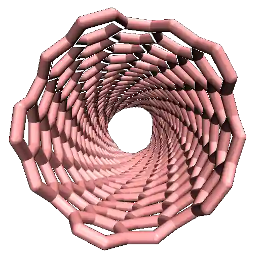
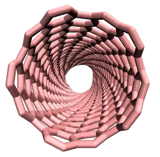
The atoms of the edges as selected within the carbon_top and carbon_bot groups can be represented with a different color.
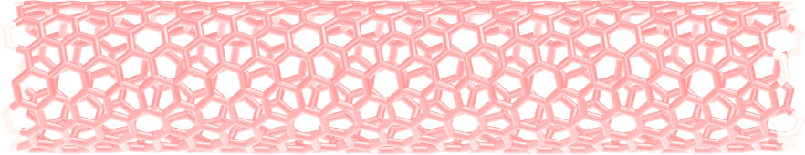
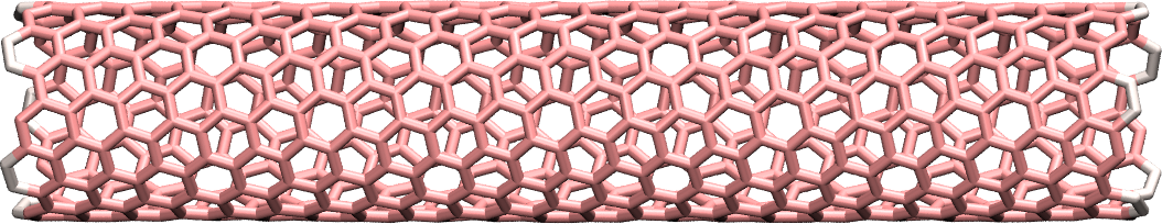
Figure: CNT with the atoms from the carbon_mid group in pink, and the atoms from the carbon_top and the carbon_bot groups in white.
When running a simulation, the number of atoms in each group is printed in the terminal (and in the log.lammps file). Always make sure that the number of atoms in each group corresponds to what is expected, just like here:
10 atoms in group carbon_top
10 atoms in group carbon_bot
680 atoms in group carbon_mid
Finally, to start from a less ideal state and create a system with some defects, let us randomly delete a small fraction of the carbon atoms. To avoid deleting atoms that are too close to the edges, let us define a new region name rdel that starts \(2\,Å\) from the CNT edges.
variable zmax_del equal ${zmax}-2
variable zmin_del equal ${zmin}+2
region rdel block INF INF INF INF ${zmin_del} ${zmax_del}
group rdel region rdel
delete_atoms random fraction 0.02 no rdel NULL 482793 bond yes
The delete_atoms command randomly deletes \(2\,\%\) of the atoms from the rdel group (i.e. about 10 atoms).
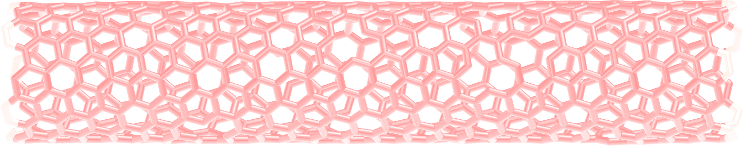
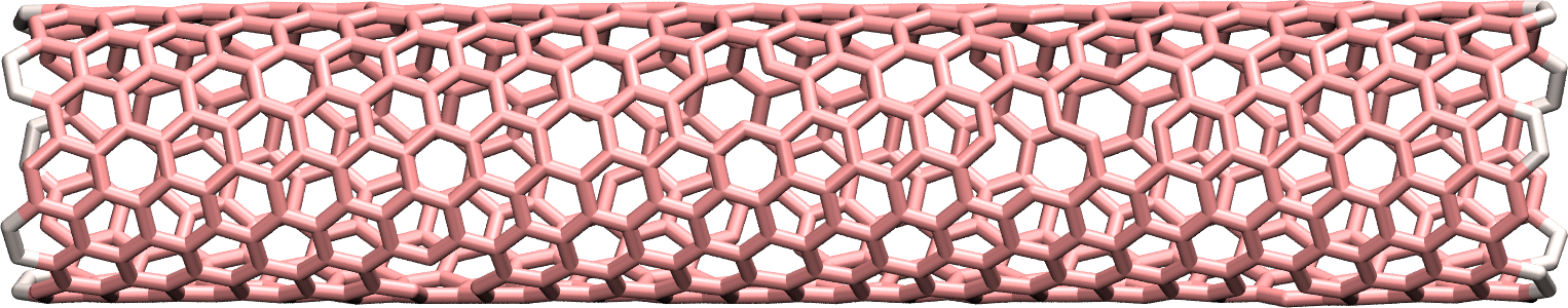
Figure: CNT with 10 randomly deleted atoms. The 10 deleted atoms were chosen randomly from the central part of the CNT.
The molecular dynamics
Let us specify the thermalization and the dynamics of the system. Add the following lines into input.lammps:
reset_atoms id sort yes
velocity carbon_mid create ${T} 48455 mom yes rot yes
fix mynve all nve
compute Tmid carbon_mid temp
fix myber carbon_mid temp/berendsen ${T} ${T} 100
fix_modify myber temp Tmid
Re-setting the atom IDs is necessary before using the velocity command, this is done by the reset_atoms command.
The velocity command gives initial velocities to the atoms of the middle group carbon_mid, ensuring an initial temperature of 300 K for these atoms with no overall translational momentum, mom yes, nor rotational momentum, rot yes.
The fix nve is applied to all atoms so that all atom positions are recalculated at every step, and a Berendsen thermostat is applied to the atoms of the group carbon_mid only [23]. The fix_modify myber ensures that the fix Berendsen uses the temperature of the group carbon_mid as an input, instead of the temperature of the whole system. This is necessary to make sure that the frozen edges won’t bias the temperature. Note that the atoms of the edges do not need a thermostat because their motion will be restrained, see below.
Deal with semi-frozen system
Always be careful when part of a system is frozen, as is the case here. When some atoms are frozen, the total temperature of the system is effectively lower than the applied temperature because the frozen atoms have no thermal motion (their temperature is therefore \(0\,\text{K}\)).
To restrain the motion of the atoms at the edges, let us add the following commands to input.lammps:
fix mysf1 carbon_top setforce 0 0 0
fix mysf2 carbon_bot setforce 0 0 0
velocity carbon_top set 0 0 0
velocity carbon_bot set 0 0 0
The two setforce commands cancel the forces applied on the atoms of the two edges, respectively. The cancellation of the forces is done at every step, and along all 3 directions of space, \(x\), \(y\), and \(z\), due to the use of 0 0 0. The two velocity commands set the initial velocities along \(x\), \(y\), and \(z\) to 0 for the atoms of carbon_top and carbon_bot, respectively.
As a consequence of these last four commands, the atoms of the edges will remain immobile during the simulation (or at least they would if no other command was applied to them).
On imposing a constant velocity to a system
The velocity set commands impose the velocity of a group of atoms at the start of a run but do not enforce the velocity during the entire simulation. When velocity set is used in combination with setforce 0 0 0, as is the case here, the atoms won’t feel any force during the entire simulation. According to the Newton equation, no force means no acceleration, meaning that the initial velocity will persist during the entire simulation, thus producing a constant velocity motion.
Data extraction
Next, in order to measure the strain and stress suffered by the CNT, let us extract the distance \(L\) between the two edges as well as the force applied on the edges.
variable L equal xcm(carbon_top,z)-xcm(carbon_bot,z)
fix at1 all ave/time 10 10 100 v_L file output_cnt_length.dat
fix at2 all ave/time 10 10 100 f_mysf1[1] f_mysf2[1] &
    file output_edge_force.dat
Let us also add a command to print the atom coordinates in a lammpstrj file every 1000 steps.
dump mydmp all atom 1000 dump.lammpstrj
Finally, let us check the temperature of the non-frozen group over time by printing it using a fix ave/time command:
fix at3 all ave/time 10 10 100 c_Tmid &
    file output_temperature_middle_group.dat
About extracting quantity from variable compute or fix
Notice that the values of the force on each edge are extracted from the two fix setforce mysf1 and mysf2, simply by calling them using f_, the same way variables are called using v_ and computes are called using c_.
Let us run a small equilibration step to bring the system to the required temperature before applying any deformation:
thermo 100
thermo_modify temp Tmid

timestep 1.0
run 5000
With the thermo_modify command, we specify to LAMMPS that we want the temperature \(T_\mathrm{mid}\) to be printed in the terminal, not the temperature of the entire system (because of the frozen edges, the temperature of the entire system is not relevant).
Let us impose a constant velocity deformation on the CNT by combining the velocity set command with previously defined fix setforce. Add the following lines in the input.lammps file, right after the last run 5000 command:
# 2*0.0005 A/fs = 0.001 A/fs = 100 m/s
velocity carbon_top set 0 0 0.0005
velocity carbon_bot set 0 0 -0.0005
run 10000
The chosen velocity for the deformation is \(100\,\text{m/s}\). The length \(L\) of the CNT increase linearly over time for \(t > 5\,\text{ps}\), as expected from the imposed constant velocity.

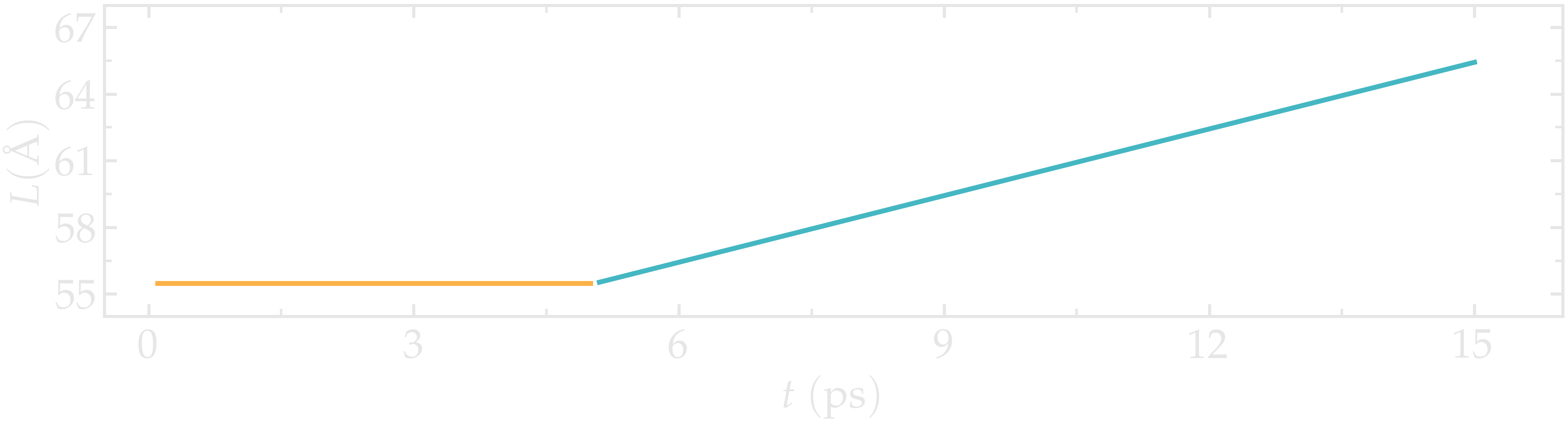
Figure: Evolution of the length \(L\) of the CNT with time. The CNT starts deforming at \(t = 5\,\text{ps}\).
The energy, which can be accessed from the log file, shows a non-linear increase with time once the deformation starts, which is expected from the typical dependency of bond energy with bond distance \(U_b = k_b \left( r - r_0 \right)^2\).
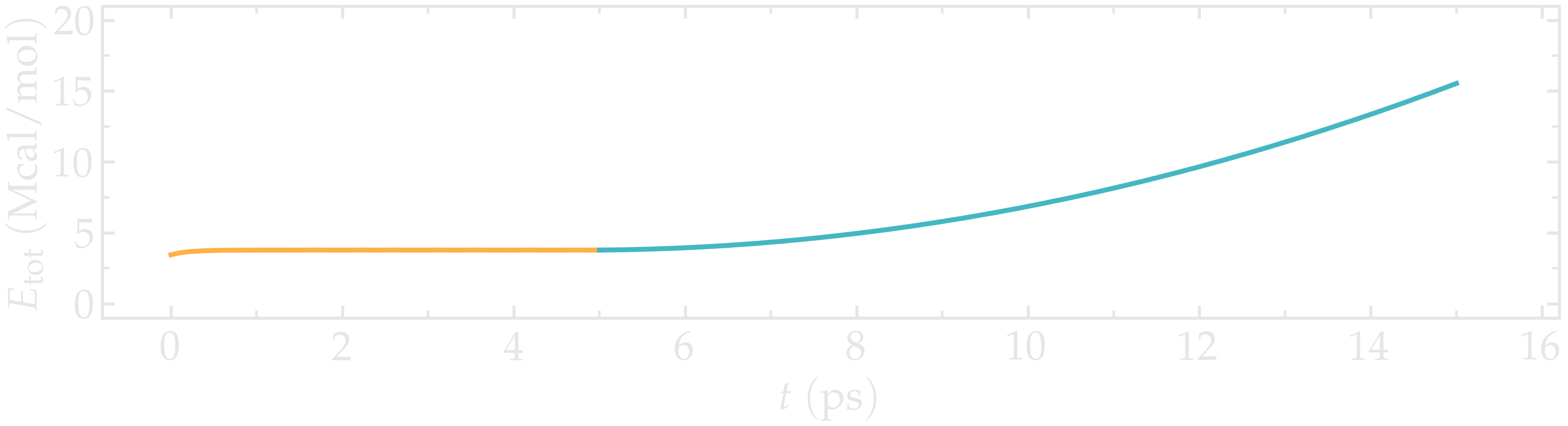

Figure: Evolution of the total energy of the system with time. The CNT starts deforming at \(t = 5\,\text{ps}\).
As always, is it important to ensure that the simulation behaves as expected by opening the dump.lammpstrj file with VMD.
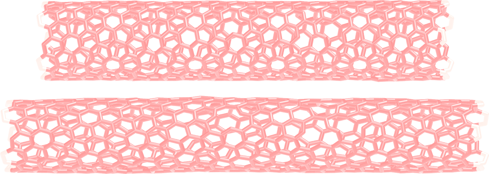
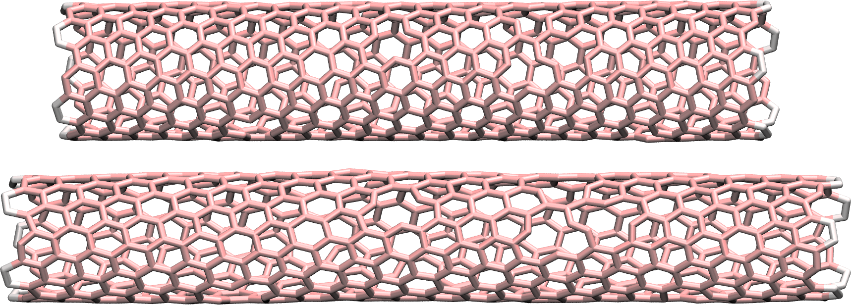
Figure: CNT before (top) and after (bottom) deformation. See the corresponding video.
Breakable bonds
When using a classical force field, as we just did, the bonds between the atoms are non-breakable. Let us perform a similar simulation and deform a small CNT again, but this time using a reactive force field that allows for the bonds to break if the applied deformation is large enough.
Input file initialization
Create a second folder named breakable-bonds/ next to unbreakable-bonds/, and create a new input file in it called input.lammps. Type into input.lammps*:
# Initialisation
variable T equal 300

units metal
atom_style atomic
boundary p p p
pair_style airebo 2.5 1 1
The first difference with the previous part is the unit system, here metal instead of real, a choice that is imposed by the AIREBO force field. A second difference is the use of the atom_style atomic instead of molecular, since no explicit bond information is required with AIREBO.
About metal units
With the metal units system of LAMMPS, the time is in pico second, distances are in Ångstrom, and the energy is in eV.
Adapt the topology file
Since bond, angle, and dihedral do not need to be explicitly set when using AIREBO, some small changes need to be made to the previously generated .data file.
Duplicate the previous file cnt_molecular.data, name the copy cnt_atom.data, and place it within breakable-bonds/. Then, remove all bond, angle, and dihedral information from cnt_atom.data. Also, remove the second column of the Atoms table, so that the cnt_atom.data looks like the following:
700 atoms
1 atom types
-40.000000 40.000000  xlo xhi
-40.000000 40.000000  ylo yhi
-12.130411 67.869589  zlo zhi

Masses

1 12.010700 # CA

Atoms # atomic

1 1 5.162323 0.464617 8.843235 # CA CNT
2 1 4.852682 1.821242 9.111212 # CA CNT
(...)
In addition, remove the Bonds table that is placed right after the Atoms table (near line 743), as well as the Angles, Dihedrals, and Impropers tables. The last lines of the file should look like this:
(...)
697 1 4.669892 -2.248901 45.824036 # CA CNT
698 1 5.099893 -0.925494 46.092010 # CA CNT
699 1 5.162323 -0.464617 47.431896 # CA CNT
700 1 5.099893 0.925494 47.699871 # CA CNT
Alternatively, you can also download the file I generate by clicking here.
Use of AIREBO potential
Then, let us import the LAMMPS data file, and set the pair coefficients by adding the following lines into input.lammps
# System definition
read_data cnt_atom.data
pair_coeff * * CH.airebo C
Here, there is one single atom type. We impose this type to be carbon by using the letter C.
Setting AIREBO pair coefficients
In the case of multiple atom types, one has to adapt the pair_coeff command. If there are 2 atom types, and both are carbon, it would read: pair_coeff * * CH.airebo C C. If atoms of type 1 are carbon and atoms of type 2 are hydrogen, then pair_coeff * * CH.airebo C H.
The CH.airebo file can be downloaded by clicking here, and must be placed within the breakable-bonds/ folder. The rest of the input.lammps is very similar to the previous one:
change_box all x final -40 40 y final -40 40 z final -60 60

group carbon_atoms type 1
variable carbon_xcm equal -1*xcm(carbon_atoms,x)
variable carbon_ycm equal -1*xcm(carbon_atoms,y)
variable carbon_zcm equal -1*xcm(carbon_atoms,z)
displace_atoms carbon_atoms move ${carbon_xcm} ${carbon_ycm} ${carbon_zcm}

variable zmax equal bound(carbon_atoms,zmax)-0.5
variable zmin equal bound(carbon_atoms,zmin)+0.5
region rtop block INF INF INF INF ${zmax} INF
region rbot block INF INF INF INF INF ${zmin}
region rmid block INF INF INF INF ${zmin} ${zmax}

group carbon_top region rtop
group carbon_bot region rbot
group carbon_mid region rmid

variable zmax_del equal ${zmax}-2
variable zmin_del equal ${zmin}+2
region rdel block INF INF INF INF ${zmin_del} ${zmax_del}
group rdel region rdel
delete_atoms random fraction 0.02 no rdel NULL 482793

reset_atoms id sort yes
velocity carbon_mid create ${T} 48455 mom yes rot yes
fix mynve all nve
compute Tmid carbon_mid temp
fix myber carbon_mid temp/berendsen ${T} ${T} 0.1
fix_modify myber temp Tmid
Note that a large distance of 120 Ångstroms was used for the box size along the z axis, to allow for larger deformation. In addition, the change_box command was placed before the displace_atoms to avoid having the CNT crossing the edge of the box.
Start the simulation
Here, let us impose a constant velocity deformation using the atoms of one edge while maintaining the other edge fixed (note that for the unbreakable CNT, the motion was imposed on the 2 edges).
First, as an equilibration step, let us set the velocity to 0 for the atoms of both edges. Let us fully constrain the edges. Add the following lines into LAMMPS:
fix mysf1 carbon_bot setforce 0 0 0
fix mysf2 carbon_top setforce 0 0 0
velocity carbon_bot set 0 0 0
velocity carbon_top set 0 0 0

variable L equal xcm(carbon_top,z)-xcm(carbon_bot,z)
fix at1 all ave/time 10 10 100 v_L file output_cnt_length.dat
fix at2 all ave/time 10 10 100 f_mysf1[1] f_mysf2[1] &
    file output_edge_force.dat

dump mydmp all atom 1000 dump.lammpstrj

thermo 100
thermo_modify temp Tmid

timestep 0.0005
run 5000
Note the relatively small timestep of \(0.0005\,\text{ps}\) used. A reactive force field usually requires a smaller timestep than a classical one. When running input.lammps with LAMMPS, you can see that the temperature deviates from the target temperature of \(300\,\text{K}\) at the start of the equilibration, but that after a few steps, it reaches the target value:
Step  Temp           E_pair         E_mol          TotEng         Press
0     300           -5084.7276      0             -5058.3973     -1515.7017
100   237.49462     -5075.4114      0             -5054.5671     -155.05545
200   238.86589     -5071.9168      0             -5050.9521     -498.15029
300   220.04074     -5067.1113      0             -5047.7989     -1514.8516
400   269.23434     -5069.6565      0             -5046.0264     -174.31158
500   274.92241     -5068.5989      0             -5044.4696     -381.28758
600   261.91841     -5065.985       0             -5042.9971     -1507.5577
700   288.47709     -5067.7301      0             -5042.4111     -312.16669
800   289.85177     -5066.5482      0             -5041.1086     -259.84893
900   279.34891     -5065.0216      0             -5040.5038     -1390.8508
1000  312.27343     -5067.6245      0             -5040.217      -465.74352
(...)
Launch the deformation
After equilibration, let us set the velocity to 15 m/s and run for a longer duration than previously. Add the following lines into input.lammps:
# 0.15 A/ps = 15 m/s
velocity carbon_top set 0 0 0.15
run 280000
The CNT should break around step 250000. If not, use a longer run.
By opening the lammpstrj file using VMD, it is possible to observe the bonds breaking at approximately two-thirds of the simulation. If the bonds do not break, use a longer run.
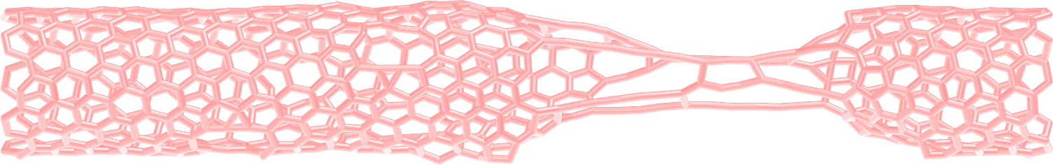
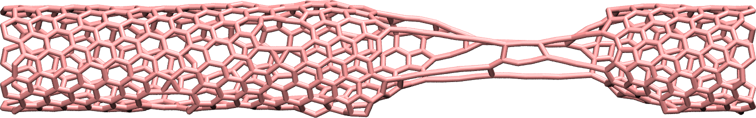
Figure: CNT with broken bonds. See the corresponding video.
About bonds in VMD
Note that VMD guesses bonds based on the distances between atoms, and not based on the presence of actual bonds between atoms in the LAMMPS simulation. Therefore the bonds seen in VMD when using the DynamicBonds representation can be misleading.
Looking at the evolution of energy again, one can see that the energy is increasing with the deformation. When bonds break, the energy relaxes abruptly, as can be seen near $t=210~text{ps}$ when plotting the evolution of the total energy with time.

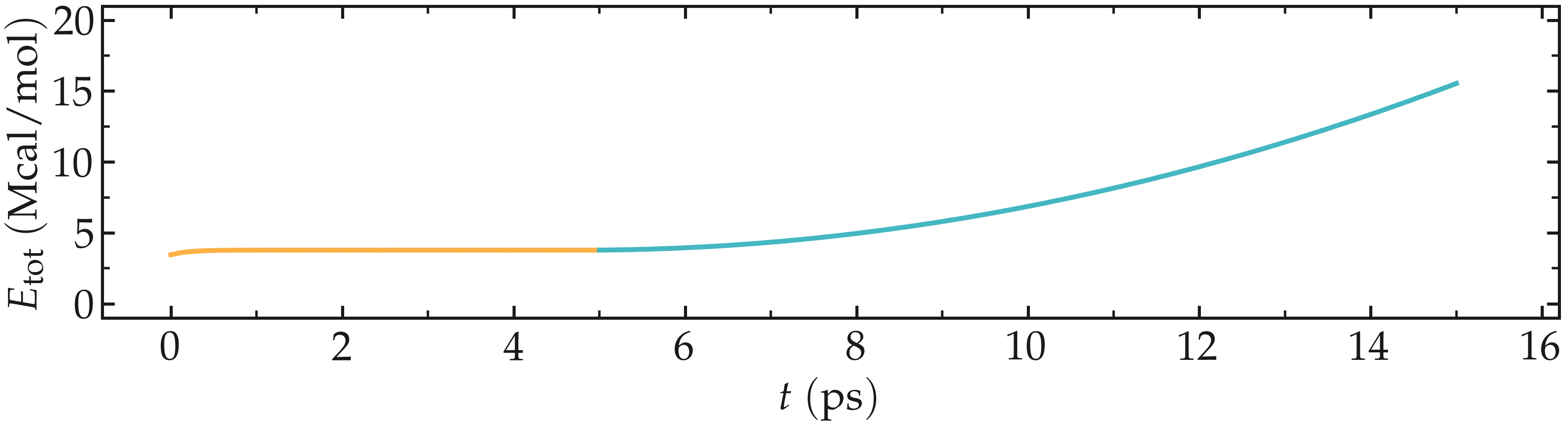
Figure: Evolution of the total energy of the system with time.
You can access the input scripts and data files that are used in these tutorials from this Github repository. This repository also contains the full solutions to the exercises.
There is a follow-up to this CNT tutorial as MDAnalysis tutorials, where a post-mortem analysis is performed using Python.
Going further with exercises
Each exercise comes with a proposed solution, see Solutions to the exercises.
Plot the strain-stress curves
Adapt the current scripts and extract the strain-stress curves for the two breakable and unbreakable CNTs:
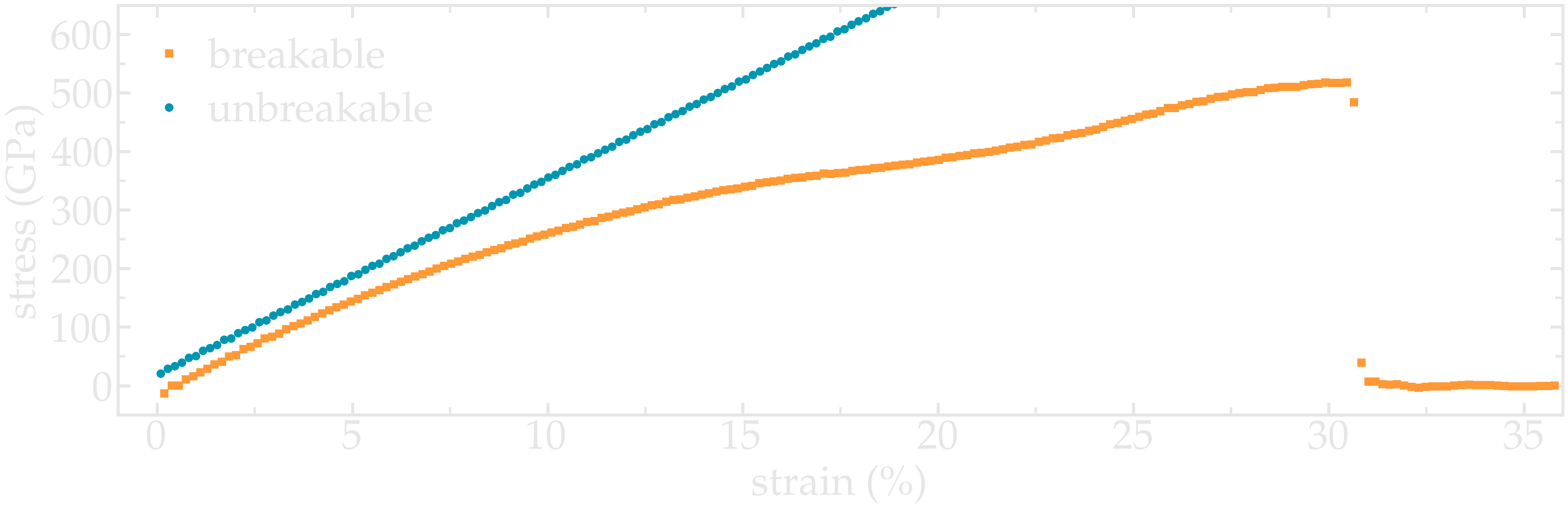
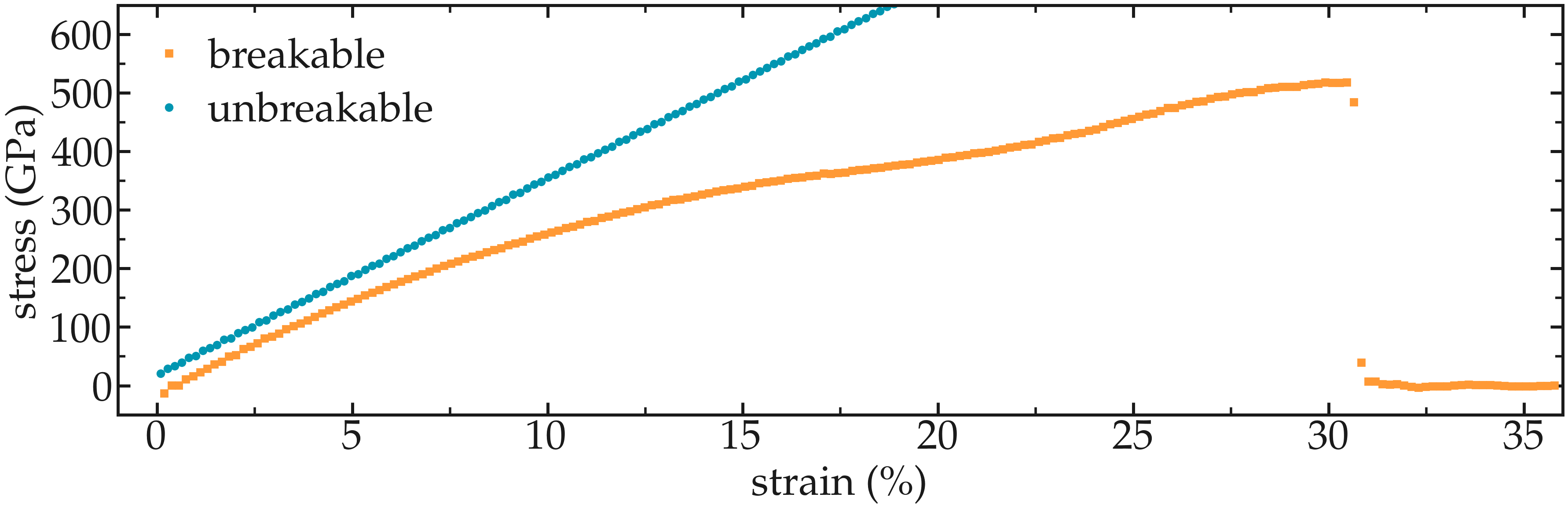
Figure: Strain-stain curves for the two CNTs, breakable and unbreakable.
Solve the flying ice cube artifact
The flying ice cube effect is one of the most famous artifacts of molecular simulations [24]. Download this seemingly simple input, which is a simplified version of the input from the first part of the tutorial. Run the input with this data file and this parameter file.
When you run this simulation using LAMMPS, you should see that the temperature is very close to \(300\,\text{K}\), as expected.
Step   Temp        E_pair      E_mol       TotEng      Press
0      327.4142    589.20707   1980.6012   3242.2444   60.344754
1000   300.00184   588.90015   1980.9013   3185.9386   51.695282
(...)
However, if you look at the system using VMD, the atoms are not moving.
Can you identify the origin of the issue, and fix the input?
Insert gas in the carbon nanotube
Modify the input from the unbreakable CNT, and add atoms of argon within the CNT.
Use the following pair_coeff for the argon, and a mass of 39.948:
pair_coeff 2 2 0.232 3.3952
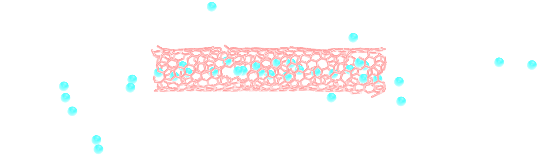
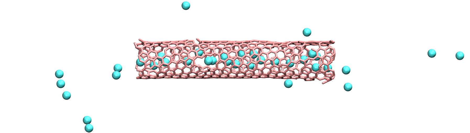
Figure: Argon atoms in a CNT. See the corresponding video.
Make a membrane of CNTs
Replicate the CNT along the x and y direction, and equilibrate the system to create an infinite membrane made of multiple CNTs.
Apply a shear deformation along xy.
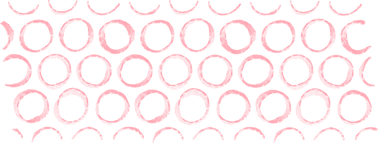

Figure: Multiple carbon nanotubes forming a membrane.
Hint
The box must be converted to triclinic to support deformation along xy.