Lennard-Jones fluid
The very basics of LAMMPS through a simple example
The objective of this tutorial is to perform the simulation of a binary fluid using LAMMPS.
The system is a Lennard-Jones fluid composed of neutral particles with two different diameters, contained within a cubic box with periodic boundary conditions In this tutorial, the temperature of the system is maintained using a Langevin thermostat [12], and basic quantities are extracted from the system, including the potential and kinetic energies.
This tutorial illustrates several key ingredients of molecular dynamics simulations, such as system initialization, energy minimization, integration of the equations of motion, and trajectory visualization.
If you find these tutorials useful for your research or simulations, you can cite: A Set of Tutorials for the LAMMPS Simulation Package by Simon Gravelle, Jacob R. Gissinger, and Axel Kohlmeyer (2025) [13]. You can access the full paper on arXiv.
This tutorial is compatible with the 2Aug2023 LAMMPS version.
My first input
To run a simulation using LAMMPS, one needs to write a series of commands in an input script. For clarity, the input scripts written for this first tutorial will be divided into five categories which we are going to fill up one by one.
Create a folder, call it my-first-input/, and then create a blank text file in it called input.lammps. Copy the following lines in input.lammps, where a line starting with a hash symbol (#) is a comment ignored by LAMMPS:
# PART A - ENERGY MINIMIZATION
# 1) Initialization
# 2) System definition
# 3) Simulation settings
# 4) Visualization
# 5) Run
These five categories are not required in every input script, and should not necessarily be in that exact order. For instance, parts 3 and 4 could be inverted, or part 4 could be omitted. Note however that LAMMPS reads input files from top to bottom, therefore the Initialization and System definition categories must appear at the top of the input, and the Run category at the bottom.
System initialization
In the first section of the script, called Initialization, let us indicate to LAMMPS the most basic information about the simulation, such as:
the conditions at the boundaries of the box (e.g. periodic or non-periodic),
the type of atoms (e.g. uncharged single dots or spheres with angular velocities).
Enter the following lines in input.lammps:
# 1) Initialization
units lj
dimension 3
atom_style atomic
pair_style lj/cut 2.5
boundary p p p
The first line, units lj, indicates that we want to use the unit system called LJ (Lennard-Jones), in which all quantities are unitless.
About Lennard-Jones (LJ) units
Lennard-Jones (LJ) units are a dimensionless system of units. LJ units are often used in molecular simulations and theoretical calculations. When using LJ units:
energies are expressed in units of \(\epsilon\), where \(\epsilon\) is the depth of the potential of the LJ interaction,
distances are expressed in units of \(\sigma\), where \(\sigma\) is the distance at which the particle-particle potential energy is zero,
masses are expressed in units of the atomic mass \(m\).
All the other quantities are normalized by a combination of \(\epsilon\), \(\sigma\), and \(m\). For instance, time is expressed in units of \(\sqrt{ \epsilon / m \sigma^2}\). Find details on the LAMMPS website.
The second line, dimension 3, indicates that the simulation is 3D. The third line, atom_style atomic, that the atomic style will be used, therefore each atom is just a dot with a mass.
About the atom style
While we are keeping things as simple as possible in this tutorial, different atom_style will be used in the following tutorials. Notably, these other atom styles will allow us to create molecules, i.e. atoms with partial charges and chemical bonds. You can find the complete list of implemented atom styles from the atom style page.
The fourth line, pair_style lj/cut 2.5, indicates that atoms will be interacting through a Lennard-Jones potential with a cut-off equal to \(r_c = 2.5\) (unitless) [14, 15]:
where \(r\) is the inter-particle distance, \(\epsilon_{ij}\) is the depth of potential well that sets the interaction strength, and \(\sigma_{ij}\) is the distance parameter or particle effective size. Here, the indexes ij refer to the particle types i and j.
About Lennard-Jones potential
The Lennard-Jones potential offers a simplified representation that captures the fundamental aspects of interactions among atoms. It depicts a scenario where two particles exhibit repulsion at extremely close distances, attraction at moderate distances, and no interaction at infinite separation. The repulsive part of the Lennard-Jones potential (i.e. the term \(\propto r^{-12}\)) is associated with the Pauli exclusion principle. The attractive part (i.e. the term in \(\propto - r^{-6}\)) is linked with the London dispersion forces.
The last line, boundary p p p, indicates that the periodic boundary conditions will be used along all three directions of space (the 3 p stand for x, y, and z, respectively).
At this point, the input.lammps is a LAMMPS input script that does nothing. You can run it using LAMMPS to verify that the input contains no mistake by typing the following command in the terminal from the my-first-input/ folder:
lmp -in input.lammps
Here lmp is linked to my compiled LAMMPS version. Running the previous command should return:
LAMMPS (2 Aug 2023 - Update 1)
Total wall time: 0:00:00
In case there is a mistake in the input script, for example, if atom_stile is written instead of atom_style, LAMMPS gives you an explicit warning:
LAMMPS (2 Aug 2023 - Update 1)
ERROR: Unknown command: atom_stile  atomic (src/input.cpp:232)
Last command: atom_stile atomic
System definition
Let us fill the System definition category of the input script:
# 2) System definition
region simulation_box block -20 20 -20 20 -20 20
create_box 2 simulation_box
create_atoms 1 random 1500 341341 simulation_box
create_atoms 2 random 100 127569 simulation_box
The first line, region simulation_box (…), creates a region named simulation_box that is a block (i.e. a rectangular cuboid) that extends from -20 to 20 (no unit) along all 3 directions of space.
The second line, create_box 2 simulation_box, creates a simulation box based on the region simulation_box with 2 types of atoms.
The third line, create_atoms (…) creates 1500 atoms of type 1 randomly within the region simulation_box. The integer 341341 is a seed that can be changed in order to create different initial conditions for the simulation. The fourth line creates 100 atoms of type 2.
If you run LAMMPS, you should see the following information in the terminal:
(...)
Created orthogonal box = (-20 -20 -20) to (20 20 20)
(...)
Created 1500 atoms
(...)
Created 100 atoms
(...)
From what is printed in the terminal, it is clear that LAMMPS correctly interpreted the commands, and first created the box with desired dimensions, then 1500 atoms, and then 100 atoms.
Simulation Settings
Let us fill the Simulation Settings category section of the input script:
# 3) Simulation settings
mass 1 1
mass 2 1
pair_coeff 1 1 1.0 1.0
pair_coeff 2 2 0.5 3.0
The two first commands, mass (…), attribute a mass equal to 1 (unitless) to both atoms of type 1 and 2. Alternatively, one could have written these two commands into one single line: mass * 1, where the star symbol means all the atom types of the simulation.
The third line, pair_coeff 1 1 1.0 1.0, sets the Lennard-Jones coefficients for the interactions between atoms of type 1, respectively the energy parameter \(\epsilon_{11} = 1.0\) and the distance parameter \(\sigma_{11} = 1.0\).
Similarly, the last line sets the Lennard-Jones coefficients for the interactions between atoms of type 2, \(\epsilon_{22} = 0.5\), and \(\sigma_{22} = 3.0\).
About cross parameters
By default, LAMMPS calculates the cross coefficients between the different atom types using geometric average: \(\epsilon_{ij} = \sqrt{\epsilon_{ii} \epsilon_{jj}}\), \(\sigma_{ij} = \sqrt{\sigma_{ii} \sigma_{jj}}\). In the present case, and even without specifying it explicitly, we thus have:
\(\epsilon_{12} = \sqrt{1.0 \times 0.5} = 0.707\), and
\(\sigma_{12} = \sqrt{1.0 \times 3.0} = 1.732\).
When necessary, cross-parameters can be explicitly specified by adding the following line into the input file: pair_coeff 1 2 0.707 1.732. This can be used for instance to increase the attraction between particles of type 1 and 2, without affecting the interactions between particles of the same type.
Note that the arithmetic rule, also known as Lorentz-Berthelot rule [16, 17], where \(\epsilon_{ij} = \sqrt{\epsilon_{ii} \epsilon_{jj}}\), \(\sigma_{ij} = (\sigma_{ii}+\sigma_{jj})/2\), is more common than the geometric rule. However, neither the geometric nor the arithmetic rules are based on rigorous arguments, so here the geometric rule will do just fine.
Due to the chosen Lennard-Jones parameters, the two types of particles are given different effective diameters, as can be seen by plotting \(E_{11} (r)\), \(E_{12} (r)\), and \(E_{22} (r)\).
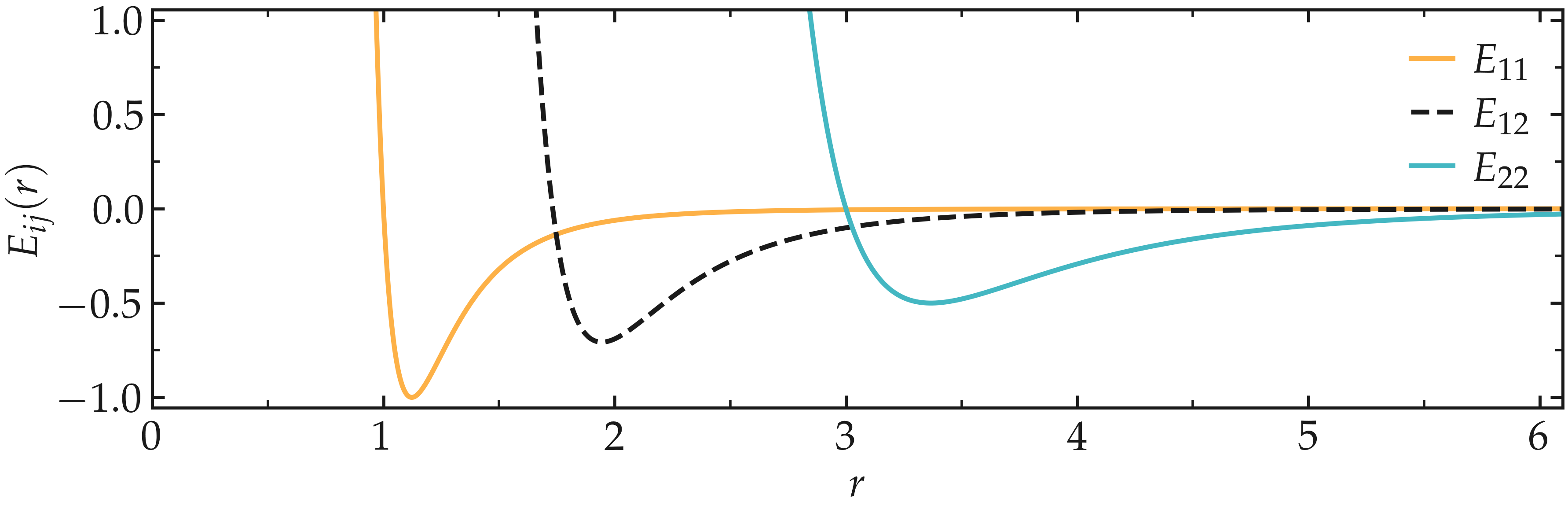
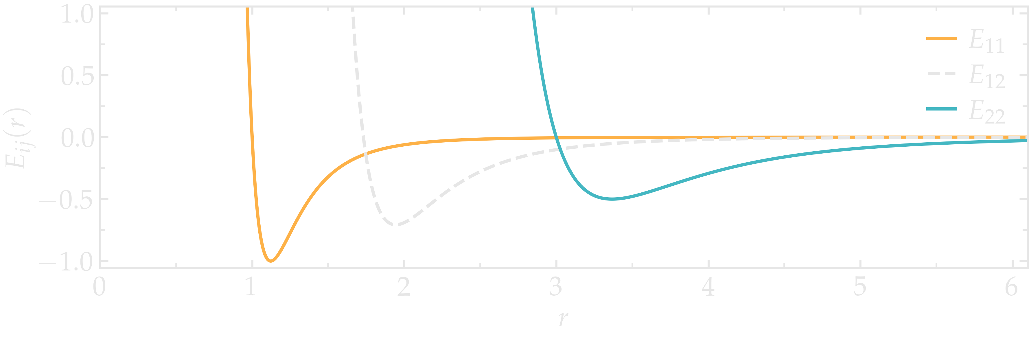
Figure: The Lennard-Jones potential \(E_{ij} (r)\) as a function of the inter-particle distance, where \(i, j = 1 ~ \text{or} ~ 2\). This figure was generated using Python with Matplotlib Pyplot, and the notebook can be accessed from Github. The Pyplot parameters used for all figures can be accessed in a dedicated repository.
Energy minimization
The system is now fully parametrized. Let us fill the two last remaining sections by adding the following lines into input.lammps:
# 4) Visualization
thermo 10
thermo_style custom step temp pe ke etotal press

# 5) Run
minimize 1.0e-4 1.0e-6 1000 10000
The thermo command asks LAMMPS to print thermodynamic information (e.g. temperature, energy) in the terminal every given number of steps, here 10 steps. The thermo_style custom requires LAMMPS to print the system temperature (temp), potential energy (pe), kinetic energy (ke), total energy (etotal), and pressure (press). Finally, the minimize command instructs LAMMPS to perform an energy minimization of the system.
About energy minimization
An energy minimization procedure consists of adjusting the coordinates of the atoms that are too close to each other until one of the stopping criteria is reached. By default, LAMMPS uses the conjugate gradient (CG) algorithm [18] (see all the other implemented methods on the min style page), which runs until one of the following criteria is reached:
The change in energy between two iterations is less than 1.0e-4.
The maximum force between two atoms in the system is lower than 1.0e-6.
The maximum number of iterations is 1000.
The maximum number of times the force and the energy have been evaluated is 10000.
Now running the simulation, we can see how the thermodynamic variables evolve as the simulation progresses:
Step  Temp  PotEng         KinEng    TotEng         Press
0     0     78840982       0         78840982       7884122
10    0     169.90532      0         169.90532      17.187291
20    0    -0.22335386     0        -0.22335386    -0.0034892297
30    0    -0.31178296     0        -0.31178296    -0.0027290466
40    0    -0.38135002     0        -0.38135002    -0.0016419218
50    0    -0.42686621     0        -0.42686621    -0.0015219081
60    0    -0.46153953     0        -0.46153953    -0.0010659992
70    0    -0.48581568     0        -0.48581568    -0.0014849169
80    0    -0.51799572     0        -0.51799572    -0.0012995545
(...)
These lines give us information about the progress of the energy minimization. First, at the start of the simulation (Step 0), the energy in the system is huge: 78840982 (unitless). This was expected because the atoms have been created at random positions within the simulation box and some of them are probably overlapping, resulting in a large initial energy which is the consequence of the repulsive part of the Lennard-Jones interaction potential. As the energy minimization progresses, the energy rapidly decreases and reaches a negative value, indicating that the atoms have been displaced at reasonable distances from each other.
On the temperature during energy minimization
As a side note, during energy minimization both temperature and kinetic energy remain equal to their initial values of 0. This is expected as the conjugate gradient algorithm only affects the positions of the particles based on the forces between them, without affecting their velocities.
Other useful information has been printed in the terminal, for example, LAMMPS tells us that the first of the four criteria to be satisfied was the energy:
Minimization stats:
Stopping criterion = energy tolerance
Molecular dynamics
The system is now ready. Let us continue by completing the input script and adding commands to perform a molecular dynamics simulation, starting from the final state of the previous energy minimization step.
Background Information – What is molecular dynamics?
Molecular dynamics (MD) is based on the numerical solution of the Newtonian equations of motion for every atom \(i\),
where \(\sum\) is the sum over all the atoms other than \(i\), \(\boldsymbol{F}_{ji}\) the force between the atom pairs \(j-i\), \(m_i\) the mass of atom \(i\), and \(\boldsymbol{a}_i\) its acceleration. The Newtonian equations are solved at every step to predict the evolution of the positions and velocities of atoms and molecules over time. Then, the velocity and position of each atom are updated according to the calculated acceleration, typically using the Verlet algorithm, or similar. More information can be found in Refs. [8, 9].
In the same input script, after the minimization command, add the following lines:
# PART B - MOLECULAR DYNAMICS
# 4) Visualization
thermo 50
Since LAMMPS reads the input from top to bottom, these lines will be executed after the energy minimization. There is no need to re-initialize or re-define the system. The thermo command is called a second time within the same input, so the previously entered value of 10 will be replaced by the value of 50 as soon as PART B starts.
Then, let us add a second Run section:
# 5) Run
fix mynve all nve
fix mylgv all langevin 1.0 1.0 0.1 1530917
timestep 0.005
run 10000
The fix nve is used to update the positions and the velocities of the atoms in the group all at every step. The group all is a default group that contains every atom.
The second fix applies a Langevin thermostat to the atoms of the group all, with a desired initial temperature of 1.0 (unitless), and a final temperature of 1.0 as well [12]. A damping parameter of 0.1 is used. The damping parameter determines how rapidly the temperature is relaxed to its desired value. The number 1530917 is a seed, you can change it to perform statistically independent simulations. Finally, the last two lines set the value of the timestep and the number of steps for the run, respectively, corresponding to a total duration of 50 (unitless).
What is a fix?
In LAMMPS, a fix is a command that performs specific tasks during a simulation, such as imposing constraints, applying forces, or modifying particle properties. Other LAMMPS-specific terms are defined in the LAMMPS Glossary.
After running the simulation, similar lines should appear in the terminal:
Step   Temp          PotEng         KinEng       TotEng        Press
388    0             -0.95476642    0           -0.95476642   -0.000304834
400    0.68476875    -0.90831467    1.0265112    0.11819648    0.023794293
500    0.97168188    -0.56803405    1.4566119    0.88857783    0.02383215
600    1.0364167     -0.44295618    1.5536534    1.1106972     0.027985679
700    1.010934      -0.39601767    1.5154533    1.1194356     0.023064983
800    0.98641731    -0.37866057    1.4787012    1.1000406     0.023131153
900    1.0074571     -0.34951264    1.5102412    1.1607285     0.023520785
(...)
The second column shows that the temperature Temp starts from 0, but rapidly reaches the requested value and stabilize itself near \(T=1\).
From what has been printed in the log file, one can plot the potential energy (\(p_\text{e}\)) and the kinetic energy (\(k_\text{e}\)) of the system over time. The potential energy, \(p_\text{e}\), rapidly decreases during energy minimization. Then, after the molecular dynamics simulation starts, \(p_\text{e}\) increases until it reaches a plateau value of about -0.25. The kinetic energy, \(k_\text{e}\), is equal to zero during energy minimization and then increases during molecular dynamics until it reaches a plateau value of about 1.5.
Figure: a) Potential energy (\(p_\text{e}\)) of the binary mixture as a function of the time \(t\). b) Kinetic energy (\(k_\text{e}\)) as a function of \(t\).
Trajectory visualization
The simulation is running well, but we would like to visualize the trajectories of the atoms. To do so, we first need to print the positions of the atoms in a file at a regular interval.
Add the following command to the input.lammps file, in the Visualization section of PART B:
dump mydmp all atom 100 dump.lammpstrj
Run the input.lammps using LAMMPS again. A file named dump.lammpstrj must appear within my-first-input/. A .lammpstrj file can be opened using VMD. With Ubuntu/Linux, you can simply execute in the terminal:
vmd dump.lammpstrj
Otherwise, you can open VMD and import the dump.lammpstrj file manually using File -> New molecule.
By default, you should see a cloud of lines, but you can improve the representation (see this VMD tutorial for basic instructions).
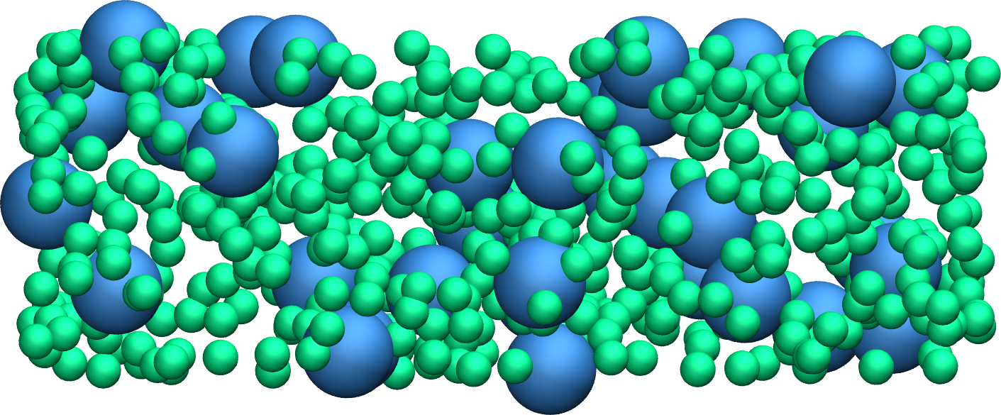
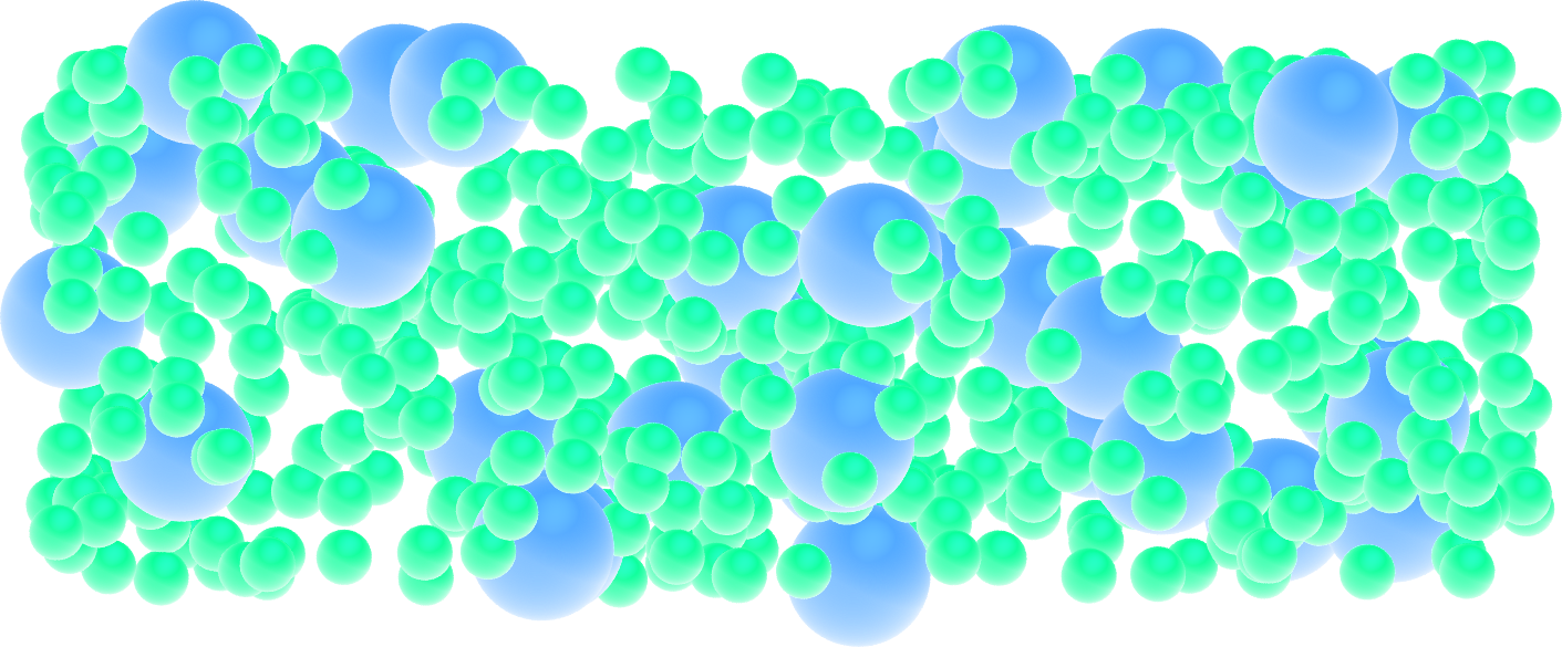
Figure: View of a slice of the system using VMD, with both types of atoms represented as spheres. See the corresponding video.
Improving the script
Let us improve the input script and perform slightly more advanced operations, such as imposing a specific initial positions to the atoms, and restarting the simulation from a previously saved configuration.
Control the initial atom positions
Create a new folder next to my-first-input/, and call it improved-input/. Then, create a new input file within improved-input/ and call it input.min.lammps.
Similarly to what has been done previously, copy the following lines into input.min.lammps:
# 1) Initialization
units lj
dimension 3
atom_style atomic
pair_style lj/cut 2.5
boundary p p p
To create the atoms of types 1 and 2 in two separate regions, let us create three separate regions: A cubic region for the simulation box and two additional regions for placing the atoms:
# 2) System definition
region simulation_box block -20 20 -20 20 -20 20
create_box 2 simulation_box
region region_cylinder_in cylinder z 0 0 10 INF INF side in
region region_cylinder_out cylinder z 0 0 10 INF INF side out
create_atoms 1 random 1000 341341 region_cylinder_out
create_atoms 2 random 150 127569 region_cylinder_in
The side in and side out keywords are used to define regions that are respectively inside and outside of the cylinder of radius 10. Then, copy similar lines as previously into input.min.lammps:
# 3) Simulation settings
mass 1 1
mass 2 1
pair_coeff 1 1 1.0 1.0
pair_coeff 2 2 0.5 3.0

# 4) Visualization
thermo 10
thermo_style custom step temp pe ke etotal press
dump mydmp all atom 10 dump.min.lammpstrj

# 5) Run
minimize 1.0e-4 1.0e-6 1000 10000
write_data minimized_coordinate.data
The main novelty, compared to the previous input script, is the write_data command. This command is used to print the final state of the simulation in a file named minimized_coordinate.data. Note that the write_data command is placed after the minimize command. This .data file will be used later to restart the simulation from the final state of the energy minimization step.
Run the input.min.lammps script using LAMMPS.
As soon as the simulation starts, a new dump file named dump.min.lammpstrj must appear in the folder. This .lammpstrj can be used to visualize the atom’s trajectories during minimization using VMD. At the end of the simulation, a file named minimized_coordinate.data is created by LAMMPS.
If you open minimized_coordinate.data with a text editor, you can see that it contains all the information necessary to restart the simulation, such as the number of atoms, the box size, the masses, and the pair_coeffs:
1150 atoms
2 atom types

-20 20 xlo xhi
-20 20 ylo yhi
-20 20 zlo zhi

Masses

1 1
2 1

Pair Coeffs # lj/cut

1 1 1
2 0.5 3
(...)
The minimized_coordinate.data file also contains the final positions of the atoms:
(...)
Atoms # atomic

970 1 4.4615279184230525 -19.88248310680258 -19.497251754277872 0 0 0
798 1 1.0773937287460968 -17.57843015813612 -19.353475858951473 0 0 0
21 1 -17.542385434367777 -16.647460269156497 -18.93914807895693 0 0 0
108 1 -15.96241088290946 -15.956274144833264 -19.016419910024062 0 0 0
351 1 0.08197850837343444 -16.852380573900156 -19.28249747472579 0 0 0
402 1 -5.270160783673711 -15.592291204068946 -19.6382667867645 0 0 0
(...)
The first five columns of the Atoms section correspond (from left to right) to the atom indexes (from 1 to the total number of atoms, 1150), the atom types (1 or 2 here), and the atoms positions \(x\), \(y\), \(z\). The last three columns are image flags that keep track of which atoms crossed the periodic boundary.
Restarting from a saved configuration
Let us create a new input file and start a molecular dynamics simulation directly from the previously saved configuration. Within improved-input/, create a new file named input.md.lammps and copy the same lines as previously:
# 1) Initialization
units lj
dimension 3
atom_style atomic
pair_style lj/cut 2.5
boundary p p p
Here, instead of creating a new region and adding atoms to it, we can simply import the previously saved configuration by adding the following command to input.md.lammps:
# 2) System definition
read_data minimized_coordinate.data
By visualizing the previously generated dump.min.lammpstrj file, you may have noticed that some atoms have moved from one region to the other during minimization. To start the simulation from a clean slate, with only atoms of type 2 within the cylinder and atoms of type 1 outside the cylinder, let us delete the misplaced atoms by adding the following commands to input.md.lammps:
read_data minimized_coordinate.data
region region_cylinder_in cylinder z 0 0 10 INF INF side in
region region_cylinder_out cylinder z 0 0 10 INF INF side out
group group_type_1 type 1
group group_type_2 type 2
group group_region_in region region_cylinder_in
group group_region_out region region_cylinder_out
group group_type_1_in intersect group_type_1 group_region_in
group group_type_2_out intersect group_type_2 group_region_out
delete_atoms group group_type_1_in
delete_atoms group group_type_2_out
The two first region commands recreate the previously defined regions, which is necessary since regions are not saved by the write_data command.
The first two group commands are used to create groups containing all the atoms of type 1 and all the atoms of type 2, respectively. The next two group commands create atom groups based on their positions at the beginning of the simulation, i.e. when the commands are being read by LAMMPS. The last two group commands create atom groups based on the intersection between the previously defined groups.
Finally, the two delete_atoms commands delete the atoms of type 1 that are located within the cylinder and the atoms of type 2 that are located outside the cylinder, respectively.
When you run the input.md.lammps input using LAMMPS, you can see in the log file how many atoms are in each group, and how many atoms have been deleted:
1000 atoms in group group_type_1
150 atoms in group group_type_2
149 atoms in group group_region_in
1001 atoms in group group_region_out
0 atoms in group group_type_1_in
1 atoms in group group_type_2_out
Deleted 0 atoms, new total = 1150
Deleted 1 atoms, new total = 1149
Add the following lines into input.md.lammps. Note the absence of Simulation settings section, because the settings are taken from the .data file.
# 4) Visualization
thermo 1000
dump mydmp all atom 1000 dump.md.lammpstrj
Let us extract the number of atoms of each type inside the cylinder as a function of time, by adding the following commands to input.md.lammps:
variable n_type1_in equal count(group_type_1,region_cylinder_in)
variable n_type2_in equal count(group_type_2,region_cylinder_in)
fix myat1 all ave/time 10 200 2000 v_n_type1_in &
    file output-population1vstime.dat
fix myat2 all ave/time 10 200 2000 v_n_type2_in &
    file output-population2vstime.dat
The two variables are used to count the number of atoms of a specific group in the region_cylinder_in region.
The two fix ave/time are calling the previously defined variables and are printing their values into text files. By using 10 200 2000, variables are evaluated every 10 steps, averaged 200 times, and printed in the .dat files every 2000 steps.
In addition to counting the atoms in each region, let us also extract the coordination number per atom between atoms of types 1 and 2. The coordination number is a measure of the average number of type 2 atoms in the vicinity of type 1 atoms, serving as a good indicator of the degree of mixing in a binary mixture. Add the following lines into input.md.lammps:
compute coor12 group_type_1 coord/atom cutoff 2.0 group group_type_2
compute sumcoor12 all reduce ave c_coor12
fix myat3 all ave/time 10 200 2000 &
    c_sumcoor12 file coordinationnumber12.dat
The compute ave is used to average the per atom coordination number that is calculated by the coord/atom compute. This averaging is necessary as coord/atom returns an array where each value corresponds to a certain couple of atoms i-j. Such an array can’t be printed by fix ave/time. Finally, let us complete the script by adding the following lines to input.md.lammps:
# 5) Run
velocity all create 1.0 4928459 mom yes rot yes dist gaussian
fix mynve all nve
fix mylgv all langevin 1.0 1.0 0.1 1530917 zero yes
timestep 0.005
run 300000
write_data mixed.data
There are a few differences from the previous simulation. First, the velocity create command attributes an initial velocity to every atom. The initial velocity is chosen so that the average initial temperature is equal to 1 (unitless). The additional keywords ensure that no linear momentum (mom yes) and no angular momentum (rot yes) are given to the system and that the generated velocities are distributed as a Gaussian. Another improvement is the zero yes keyword in the Langevin thermostat, which ensures that the total random force applied to the atoms is equal to zero.
Run input.md.lammps using LAMMPS and visualize the trajectory using VMD.
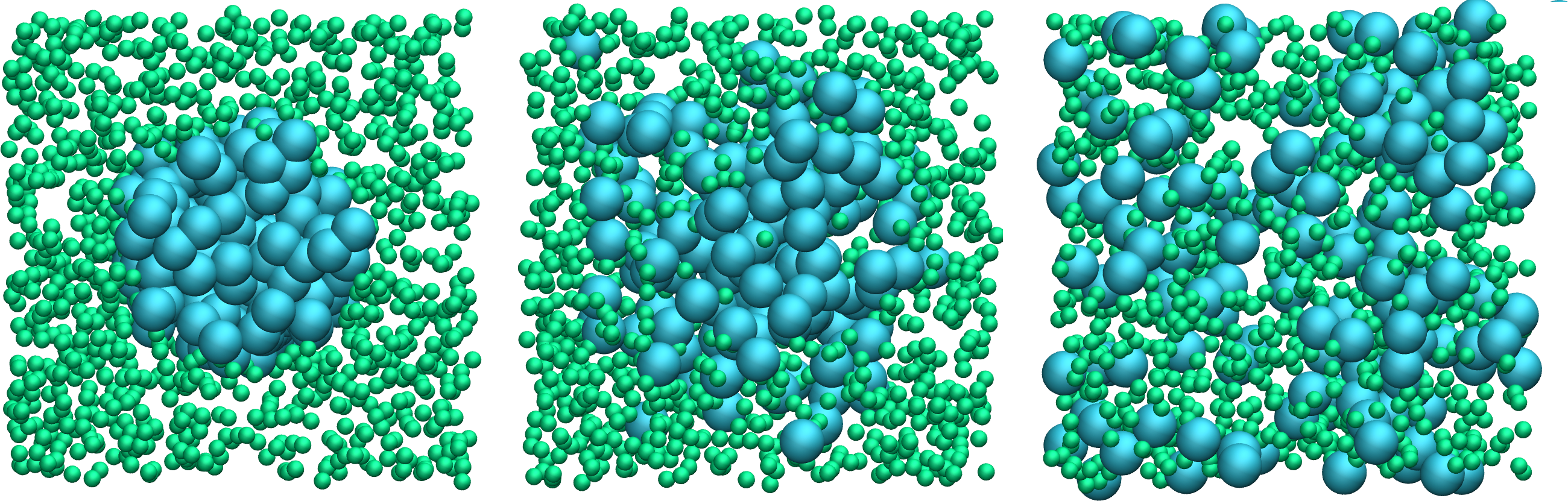
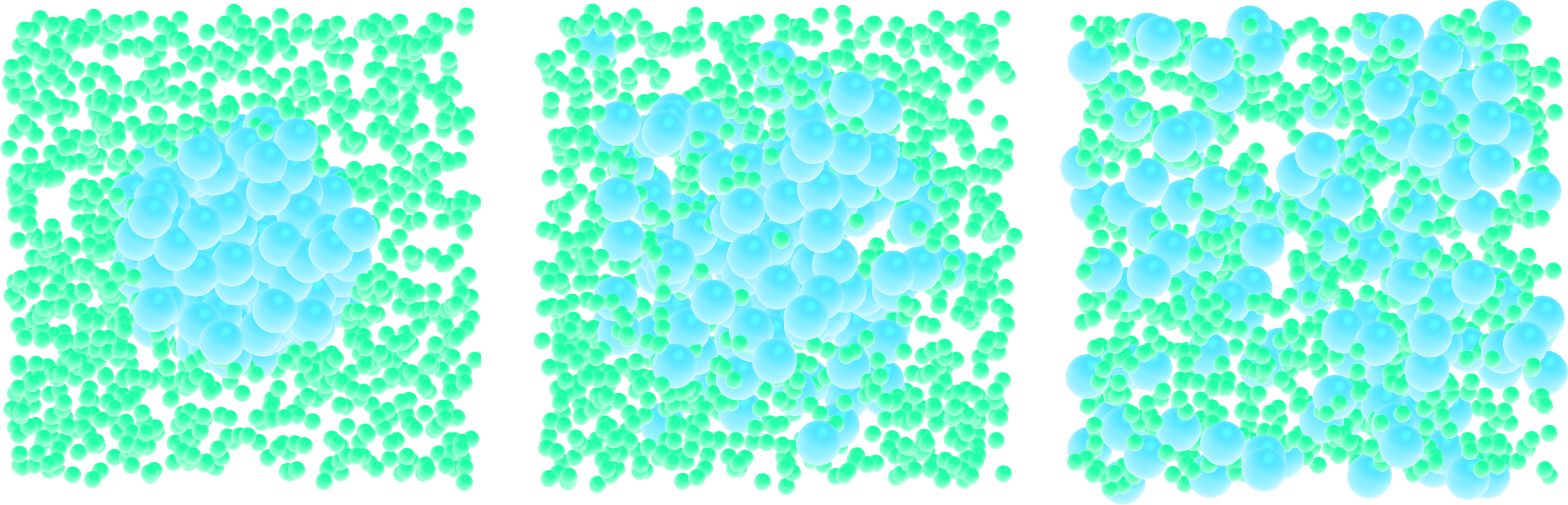
Figure: Evolution of the system during mixing. The three snapshots show respectively the system at \(t=0\) (left panel), \(t=75\) (middle panel), and \(t=1500\) (right panel).
After running input.md.lammps using LAMMPS, you can observe the number of atoms in each region from the generated data files, as well as the evolution of the coordination number due to mixing:
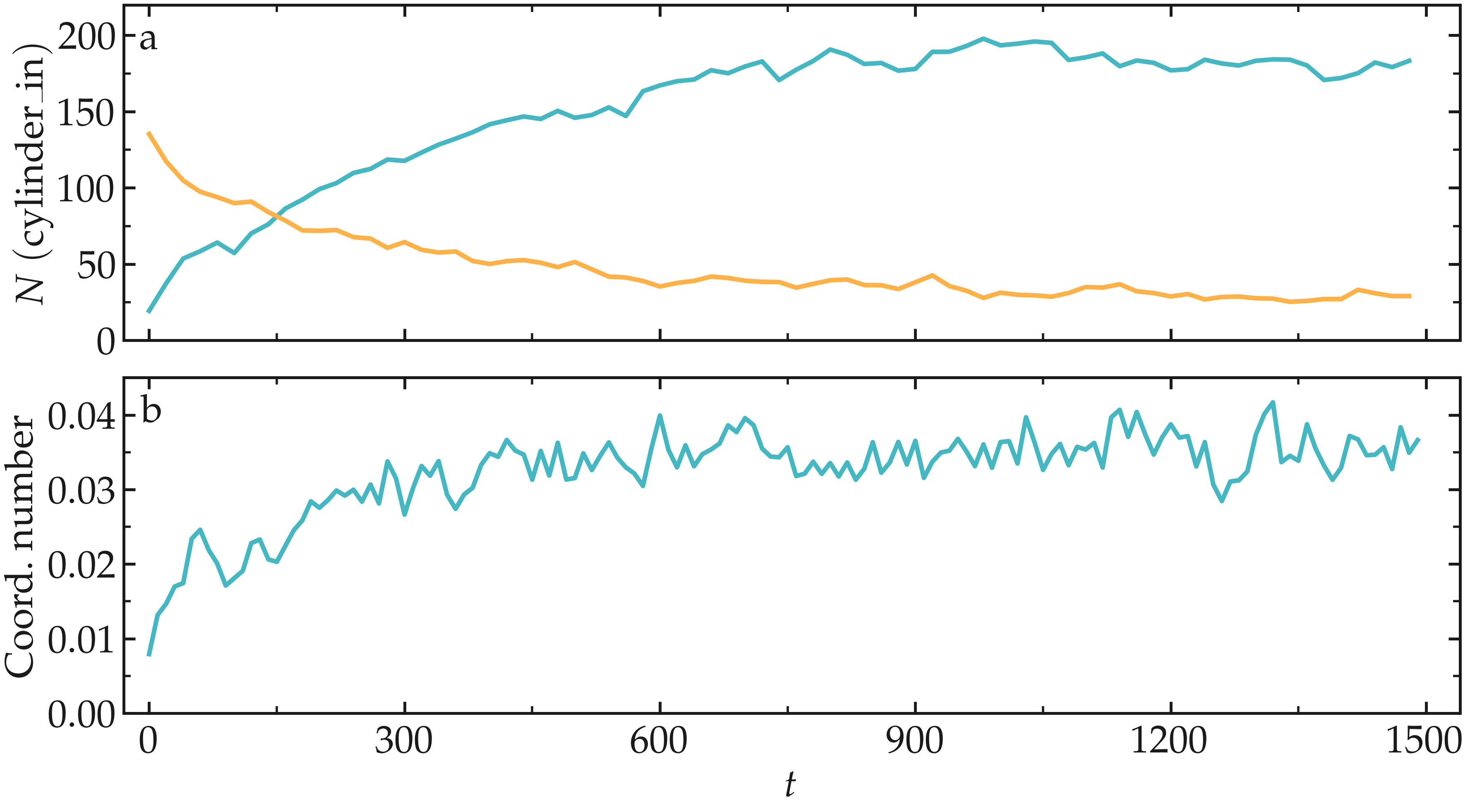
Figure: Evolution of the number of atoms within the region_cylinder_in region as a function of time (a), and evolution of the coordination number between atoms of types 1 and 2 (b).
You can access the input scripts and data files that are used in these tutorials from this Github repository. This repository also contains the full solutions to the exercises.
Going further with exercises
Each exercise comes with a proposed solution, see Solutions to the exercises.
Solve Lost atoms error
For this exercise, the following input script is provided:
units lj
dimension 3
atom_style atomic
pair_style lj/cut 2.5
boundary p p p

region simulation_box block -20 20 -20 20 -20 20
create_box 1 simulation_box
create_atoms 1 random 1000 341841 simulation_box

mass 1 1
pair_coeff 1 1 1.0 1.0

dump mydmp all atom 100 dump.lammpstrj
thermo 100
thermo_style custom step temp pe ke etotal press

fix mynve all nve
fix mylgv all langevin 1.0 1.0 0.1 1530917
timestep 0.005

run 10000
As it is, this input returns one of the most common error that you will encounter using LAMMPS:
ERROR: Lost atoms: original 1000 current 984
The goal of this exercise is to fix the Lost atoms error without using any other command than the ones already present. You can only play with the values of the parameters and/or replicate every command as many times as needed.
Note
This script is failing because particles are created randomly in space, some of them are likely overlapping, and no energy minimization is performed prior to start the molecular dynamics simulation.
Create a demixed dense phase
Starting from one of the input created in this tutorial, fine-tune the parameters such as particle numbers and interaction to create a simulation with the following properties:
the density in particles must be high,
both particles of type 1 and 2 must have the same size,
particles of type 1 and 2 must demix.
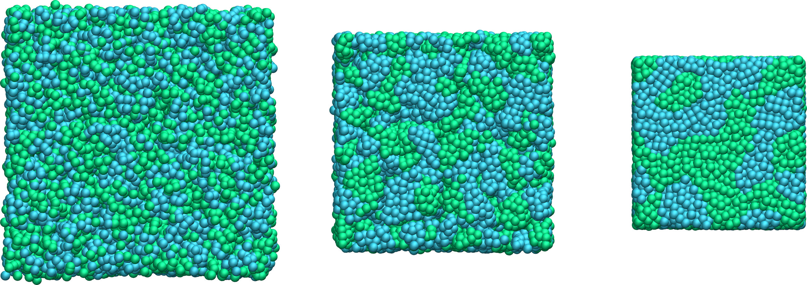
Figure: Snapshots taken at different times showing the particles of type 1 and type 2 progressively demixing and forming large demixed areas.
Hint
An easy way to create a dense phase is to allow the box dimensions to relax until the vacuum disappears. You can do that by replacing the fix nve with fix nph.
From atoms to molecules
Add a bond between particles of type 2 to create dumbbell molecules instead of single particles.
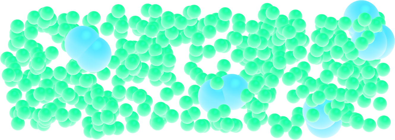
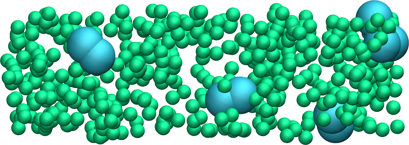
Figure: Dumbbell molecules made of 2 large spheres mixed with smaller particles (small spheres). See the corresponding video.
Similarly to the dumbbell molecules, create a small polymer, i.e. a long chain of particles linked by bonds and angles.
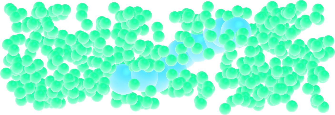
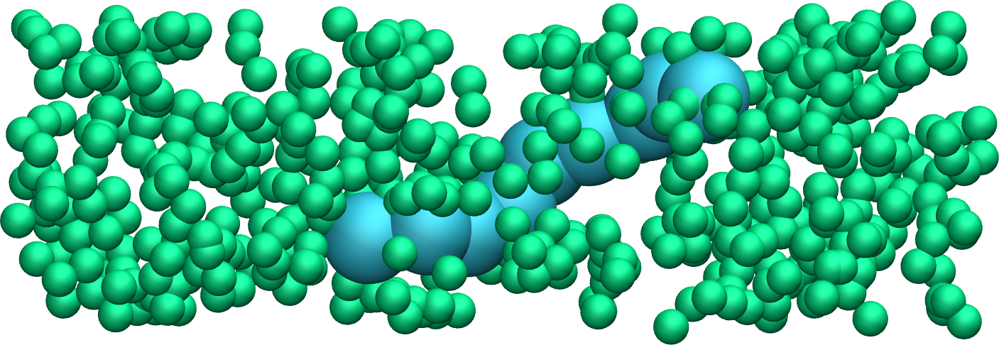
Figure: A single small polymer molecule made of 9 large spheres mixed with smaller particles. See the corresponding video.
Hints
Use a molecule template to easily insert as many atoms connected by bonds (i.e. molecules) as you want. A molecule template typically begins as follows:
2 atoms
1 bonds

Coords

1 0.5 0 0
2 -0.5 0 0

(...)
A bond section also needs to be added, see this page for details on the formatting of a molecule template.