Reactive silicon dioxide
Simulating a chemically reactive structure
The objective of this tutorial is to use a reactive force field (ReaxFF [42, 43]) to calculate the partial charges of a system undergoing deformation, as well as chemical bond formation and breaking.
The system simulated here is a block of silicon dioxide (\(\text{SiO}_2\)) that is deformed until rupture. Particular attention is given to the evolution of the atomic charges during the deformation of the structure, and the chemical reactions occurring due to the deformation are tracked over time.
If you are completely new to LAMMPS, I recommend that you follow this tutorial on a simple Lennard-Jones fluid first.
If you find these tutorials useful for your research or simulations, you can cite: A Set of Tutorials for the LAMMPS Simulation Package by Simon Gravelle, Jacob R. Gissinger, and Axel Kohlmeyer (2025) [13]. You can access the full paper on arXiv.
This tutorial is compatible with the 2Aug2023 LAMMPS version.
Prepare and relax
Create a folder, name it RelaxSilica/, and download the initial topology of a small amorphous silica structure.
About the initial structure
The system was created by temperature annealing using another force field named vashishta [44]. In case you are interested in the input creation, the files used for creating the initial topology is available here.
If you open the silica.data file, you will see in the Atoms section that all silicon atoms have the same charge \(q = 1.1\,\text{e}\), and all oxygen atoms the charge \(q = -0.55\,\text{e}\). This is common with classical force fields and will change once ReaxFF is used.
The first action we need to perform here is to relax the structure with ReaxFF, which we are gonna do using molecular dynamics. To make sure that the system equilibrates nicely, let us track some parameters over time.
Create an input file called input.lammps in RelaxSilica/, and copy the following lines into it:
units real
atom_style full

read_data silica.data

mass 1 28.0855 # Si
mass 2 15.999 # O
So far, the input is very similar to what was seen in the previous tutorials. Some basic parameters are defined (units, atom_style and masses), and the .data file is imported by the read_data command. Now, let us copy three crucial lines into the input.lammps file:
pair_style reaxff NULL safezone 3.0 mincap 150
pair_coeff * * reaxCHOFe.ff Si O
fix myqeq all qeq/reaxff 1 0.0 10.0 1.0e-6 reaxff maxiter 400
Here, the pair_style reaxff is used with no control file. The safezone and mincap keywords have been added to avoid memory allocation issues, which sometimes can trigger the segmentation faults and bondchk failed errors.
The pair_coeff uses the reaxCHOFe.ff file, which must be downloaded and saved within RelaxSilica/. For consistency with the masses and the silica.data file, the atoms of type 1 are set as silicon (Si), and the atoms of type 2 as oxygen (O).
Finally, the fix qeq/reaxff is used to perform charge equilibration [45]. The charge equilibration occurs at every step. The values 0.0 and 10.0 are the low and the high cutoffs, respectively, and \(1.0 \text{e} -6\) is a tolerance. Finally, maxiter sets an upper limit to the number of attempts to equilibrate the charge.
Note
If the charge does not properly equilibrate despite the 400 attempts, a warning will appear. Such warnings are likely to appear at the beginning of the simulation if the initial charges are too far from the equilibrium values.
Then, let us add some commands to the input.lammps file to measure the evolution of the charges during the simulation:
group grpSi type 1
group grpO type 2
variable qSi equal charge(grpSi)/count(grpSi)
variable qO equal charge(grpO)/count(grpO)
Let us also print the charge in the .log file by using thermo_style, and create a .lammpstrj file for visualization. Add the following lines into the input.lammps:
thermo 5
thermo_style custom step temp etotal press vol v_qSi v_qO
dump dmp all custom 100 dump.lammpstrj id type q x y z
Let us also use the fix reaxff/species to evaluate what species are present within the simulation. It will be useful later when the system is deformed and some bonds are broken:
fix myspec all reaxff/species 5 1 5 species.log element Si O
Here, the information will be printed every 5 steps in a file named species.log.
Let us perform a very short run using the anisotropic NPT command and relax the density of the system.
velocity all create 300.0 3482028
fix mynpt all npt temp 300.0 300.0 100 aniso 1.0 1.0 1000
timestep 0.5

run 5000

write_data silica-relaxed.data
Run the input.lammps file using LAMMPS. As seen from species.log, only one species is detected, called Si192O384, representing the entire system.
As the simulation progresses, you can see that the charges of the atoms are fluctuating since the charge of every individual atom is adjusting to its local environment in real time.
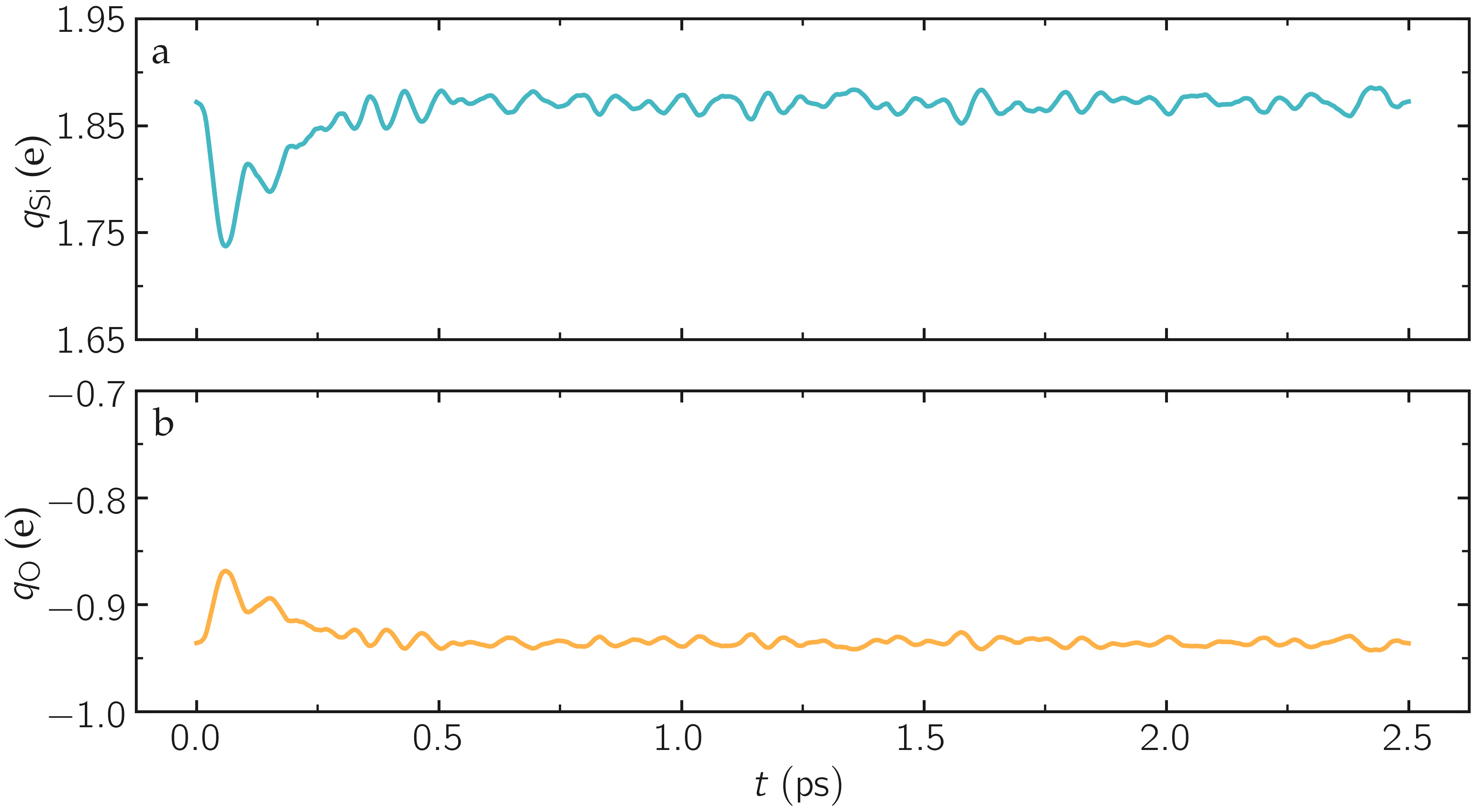
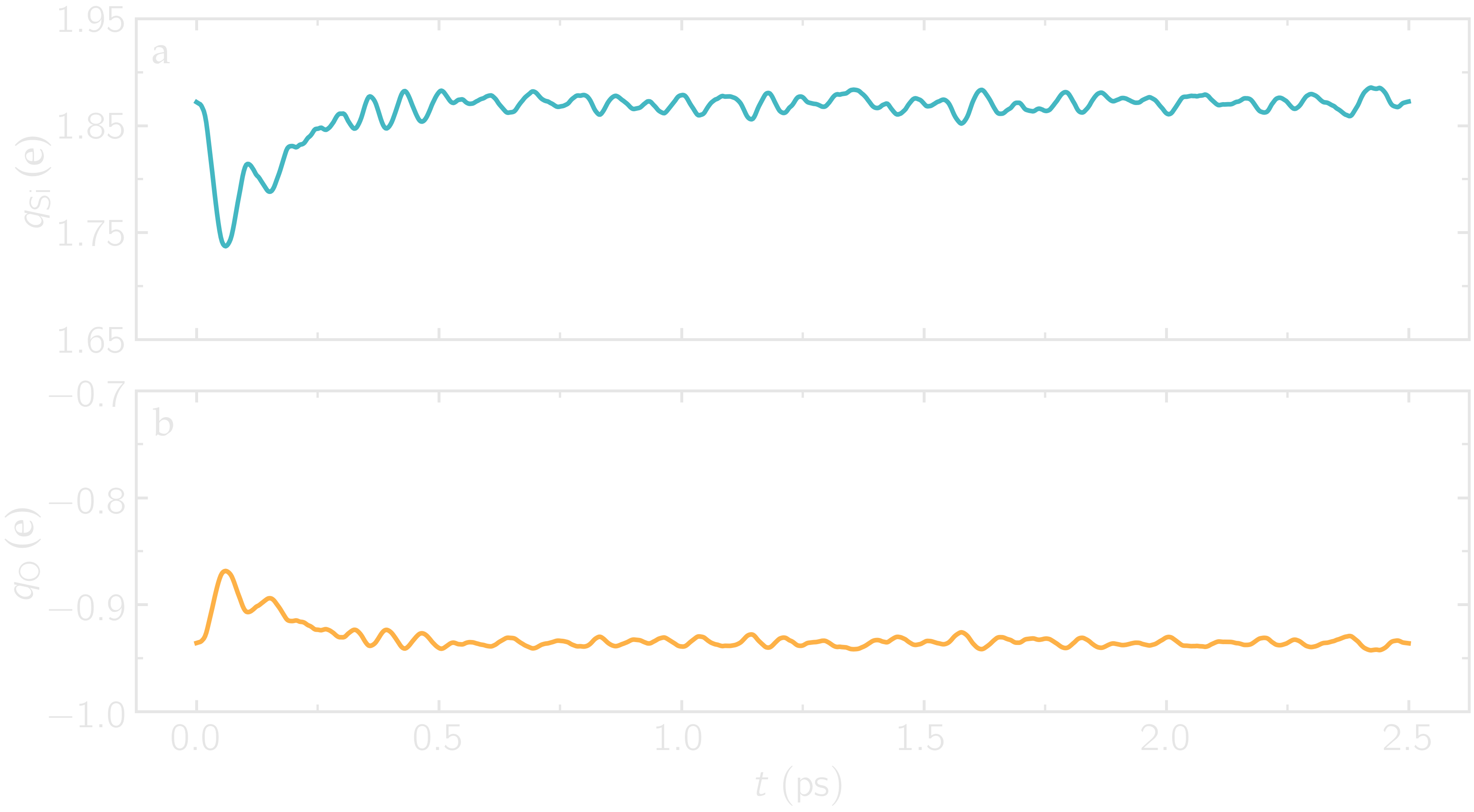
Figure: Average charge per atom of the silicon (a) and oxygen (b) atoms during equilibration, as given by the v_qSi and v_qO variables.
Additionally, the average charge of the atoms is strongly fluctuating at the beginning of the simulation. This early fluctuation correlates with a rapid volume change of the box, during which the inter-atomic distances are expected to quickly change.
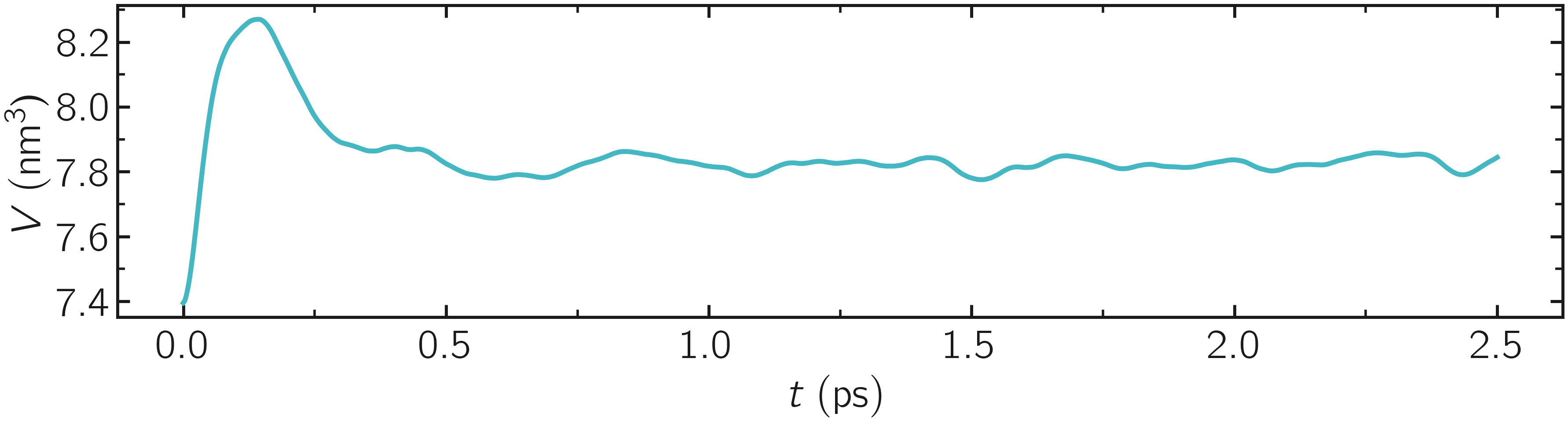
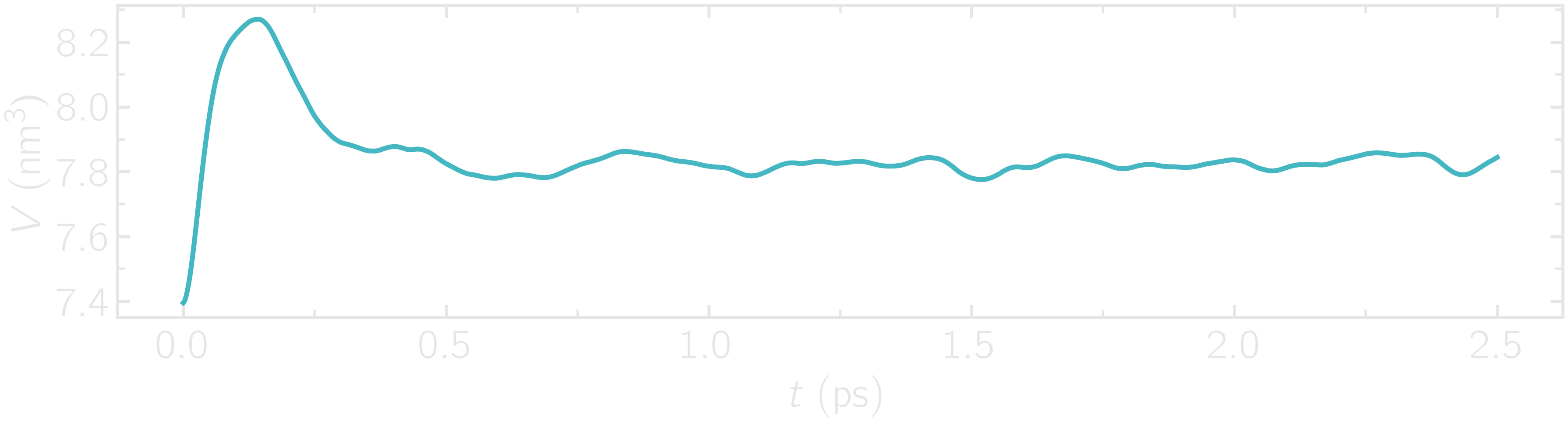
Figure: Volume of the system as a function of time.
Since each atom has a charge that depends on its local environment, the charge values are expected to be different for every atom in the system. We can plot the charge distribution \(P(q)\), using the charge values printed in the .lammptrj file.
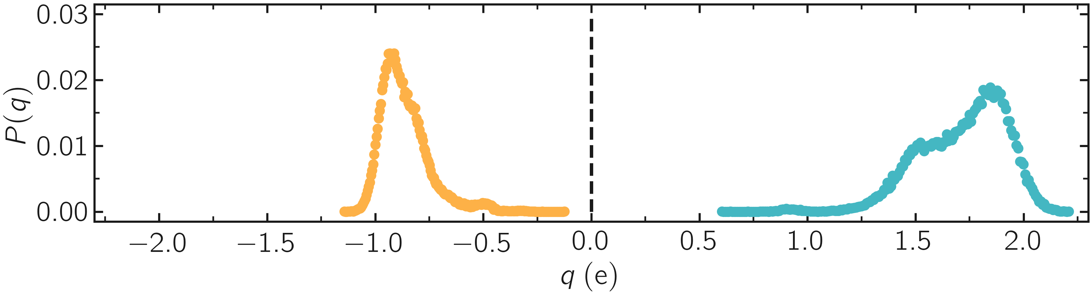
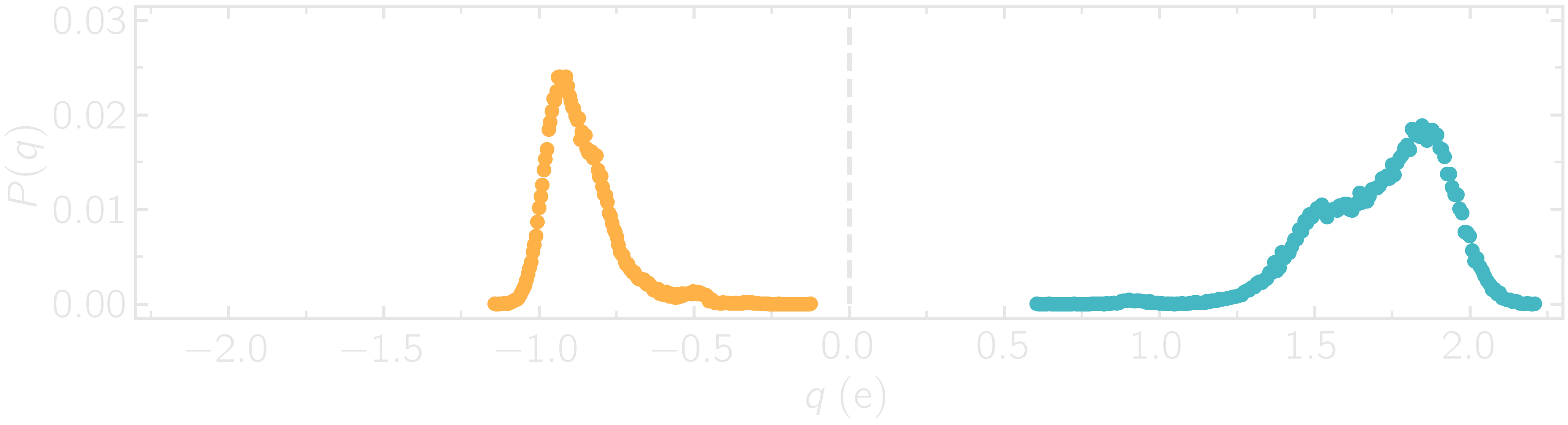
Figure: Probability distribution of charge of silicon (positive, blue) and oxygen (negative, orange) atoms during equilibration.
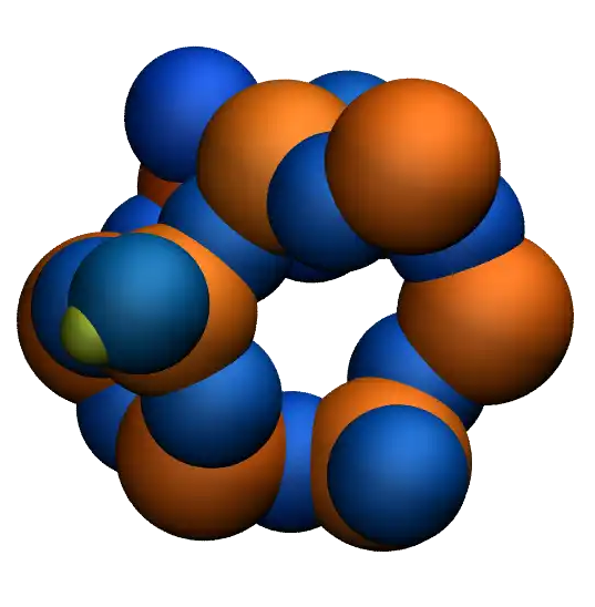
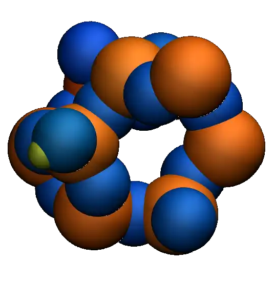
Using VMD and coloring the atoms by their charges, one can see that the atoms with the extreme-most charges are located at defects in the amorphous structure (here at the positions of the dangling oxygen groups).
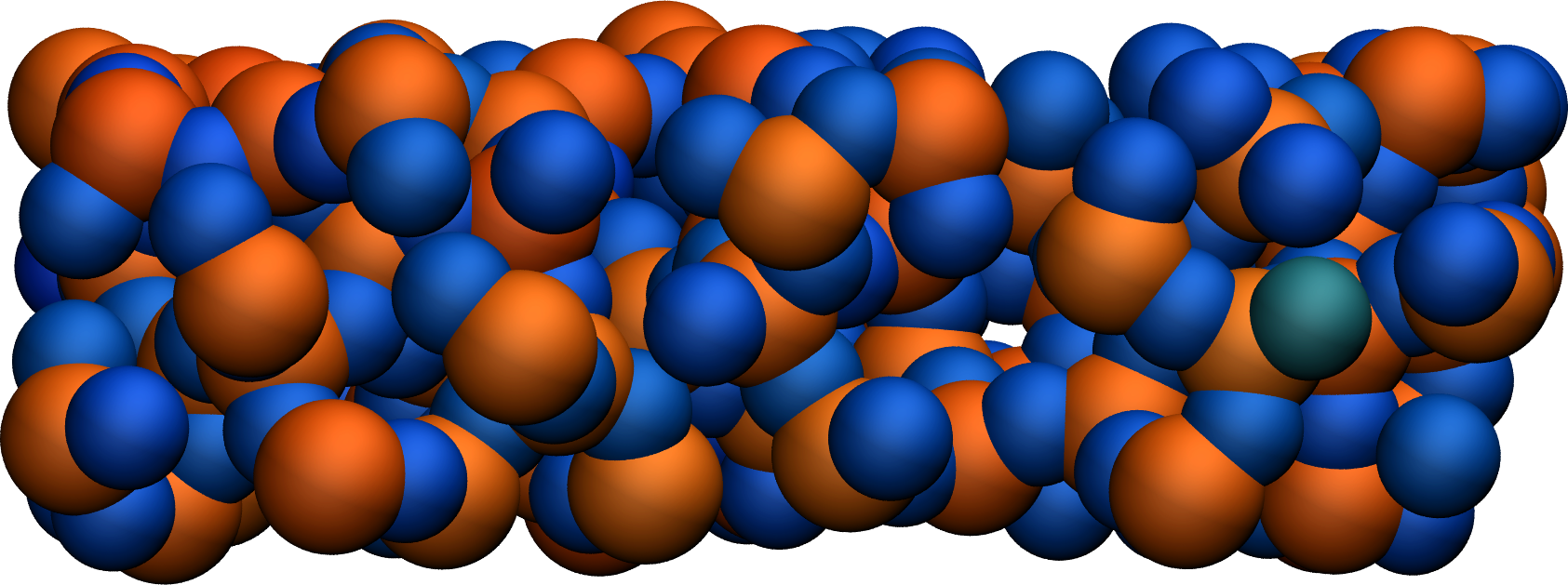
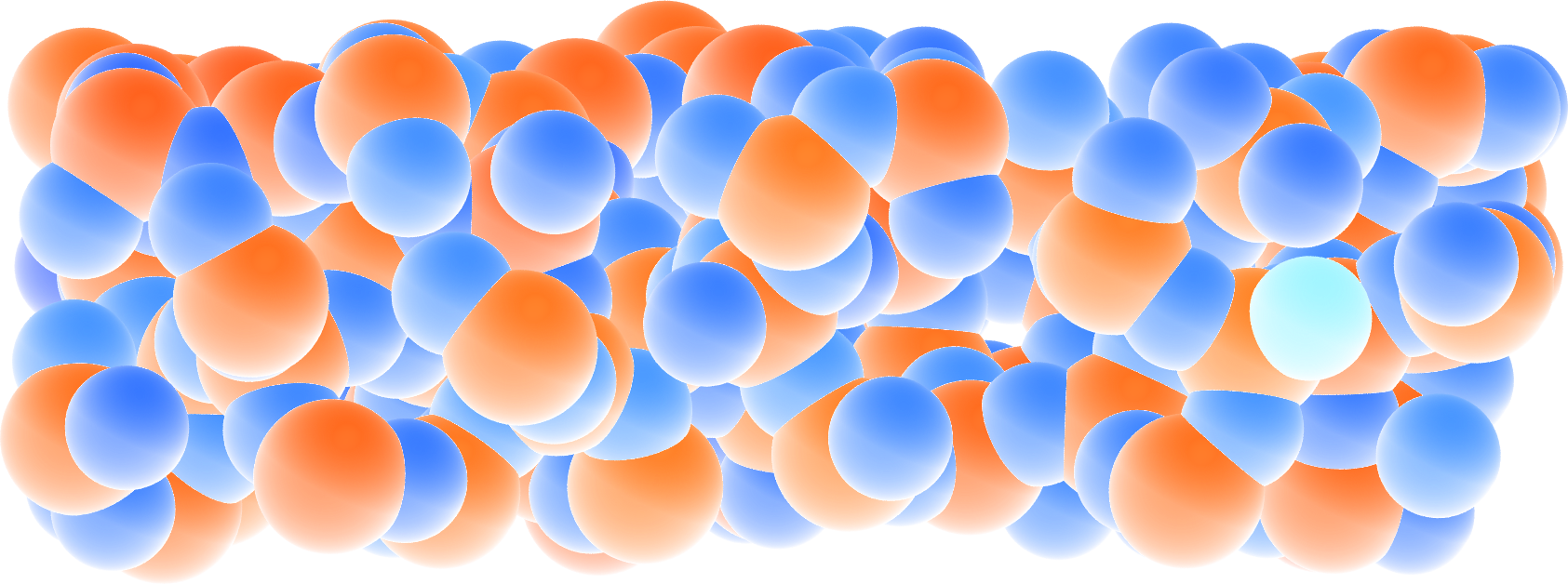
Figure: A slice of the amorphous silica, where atoms are colored by their charges. Dangling oxygen groups appear in greenish, bulk Si atoms with a charge of about \(1.8~\text{e}\) appear in red/orange, and bulk O atoms with a charge of about \(-0.9~\text{e}\) appear in blue. To color the atoms by their charge using VMD, use Charge as the coloring method in the representation windows, and then tune the Color scale in the Color control windows.
Deform the structure
Let us apply a deformation to the structure to force some \(\text{Si}-\text{O}\) bonds to break (and eventually re-assemble).
Next to RelaxSilica/, create a folder, call it Deform/ and create a file named input.lammps in it. Copy the same lines as previously in input.lammps:
units real
atom_style full

read_data ../RelaxSilica/silica-relaxed.data

mass 1 28.0855 # Si
mass 2 15.999 # O

pair_style reaxff NULL safezone 3.0 mincap 150
pair_coeff * * ../RelaxSilica/reaxCHOFe.ff Si O
fix myqeq all qeq/reaxff 1 0.0 10.0 1.0e-6 reaxff maxiter 400
The only differences with the previous input.lammps file are the paths to the .data and .ff files located within RelaxSilica/. Copy the following lines as well:
group grpSi type 1
group grpO type 2
variable qSi equal charge(grpSi)/count(grpSi)
variable qO equal charge(grpO)/count(grpO)

thermo 5
thermo_style custom step temp etotal press vol v_qSi v_qO
dump dmp all custom 100 dump.lammpstrj id type q x y z

fix myspec all reaxff/species 5 1 5 species.log element Si O
Then, let us use fix nvt instead of fix npt to apply a thermostat but no barostat:
fix mynvt all nvt temp 300.0 300.0 100
timestep 0.5
Note
Here, no barostat is used because the box volume will be imposed by the fix deform.
Let us run for 5000 steps without deformation, then apply the fix deform for elongating progressively the box along x during 25000 steps. Add the following line to input.lammps:
run 5000

fix mydef all deform 1 x erate 5e-5

run 25000

write_data silica-deformed.data
Run the input.lammps file using LAMMPS. During the deformation, the charge values progressively evolve until the structure eventually breaks down. After the structure breaks down, the charges equilibrate near new average values that differ from the starting averages. The difference between the initial and the final charges can be explained by the presence of defects as well as new solid/vacuum interfaces, and the fact that surface atoms typically have different charges compared to bulk atoms.
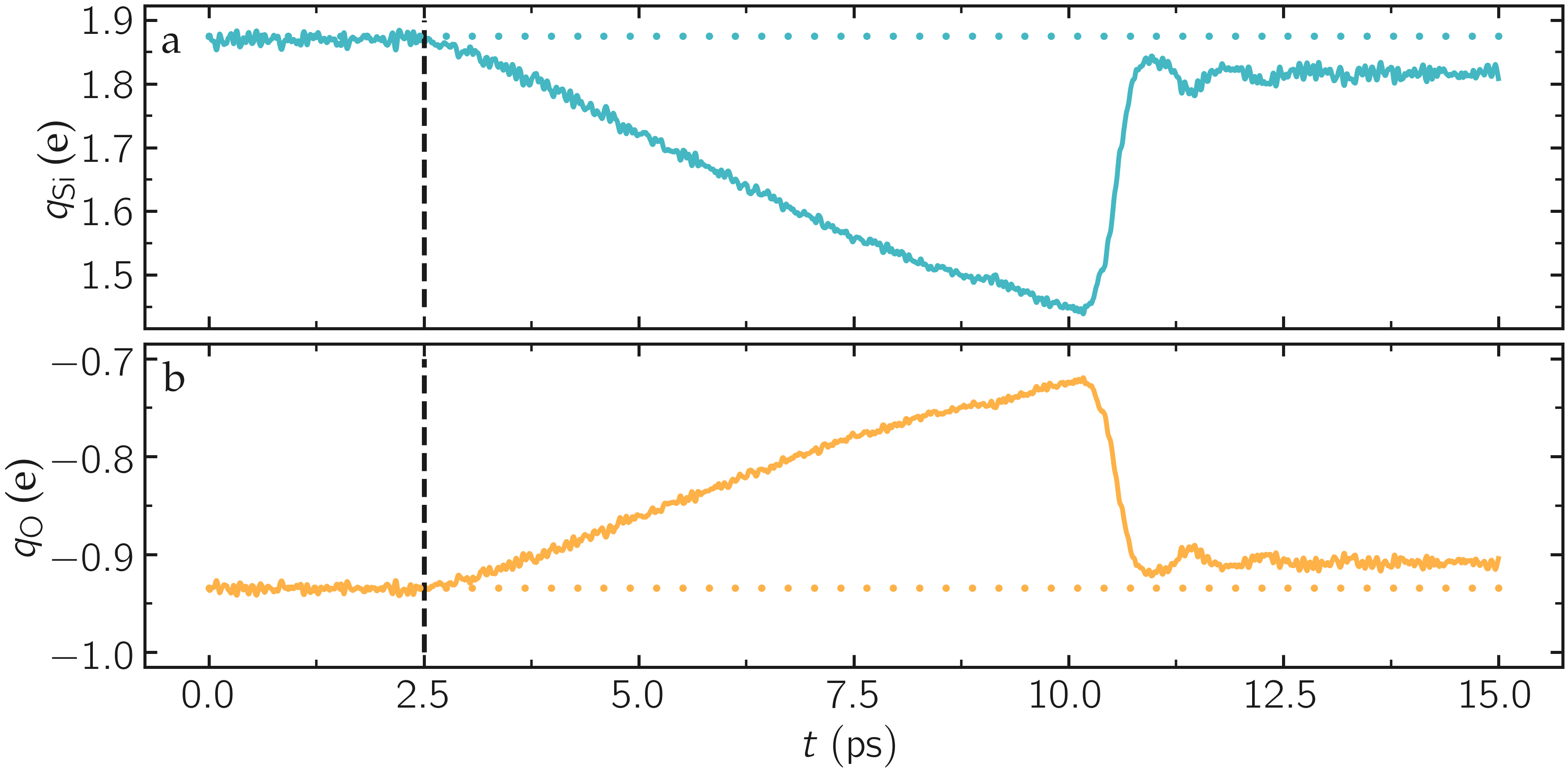
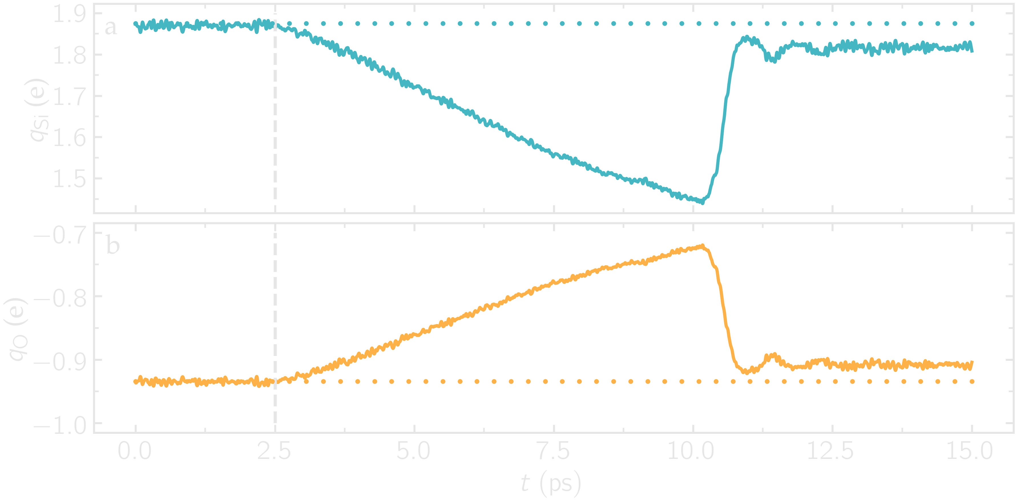
Figure: Evolution of the average charge per atom of the silicon \(q_\text{Si}\) (a) and oxygen \(q_\text{O}\) (b) over time \(t\). The vertical dashed lines mark the beginning of the deformation, and the horizontal dashed lines denote the initial values for the average charge.
There is also a strong increase in temperature during the rupture of the material.
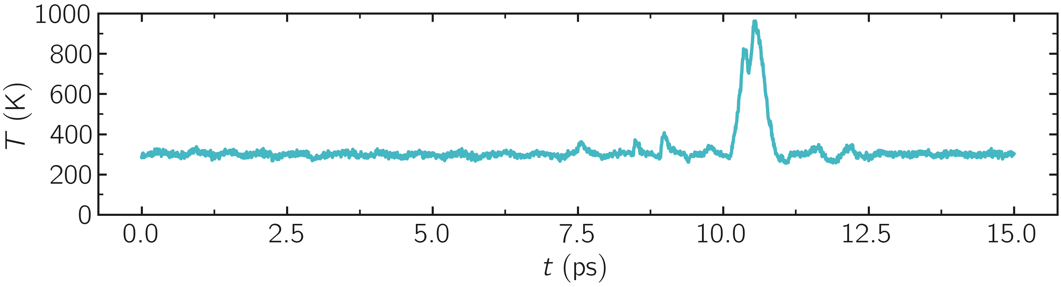
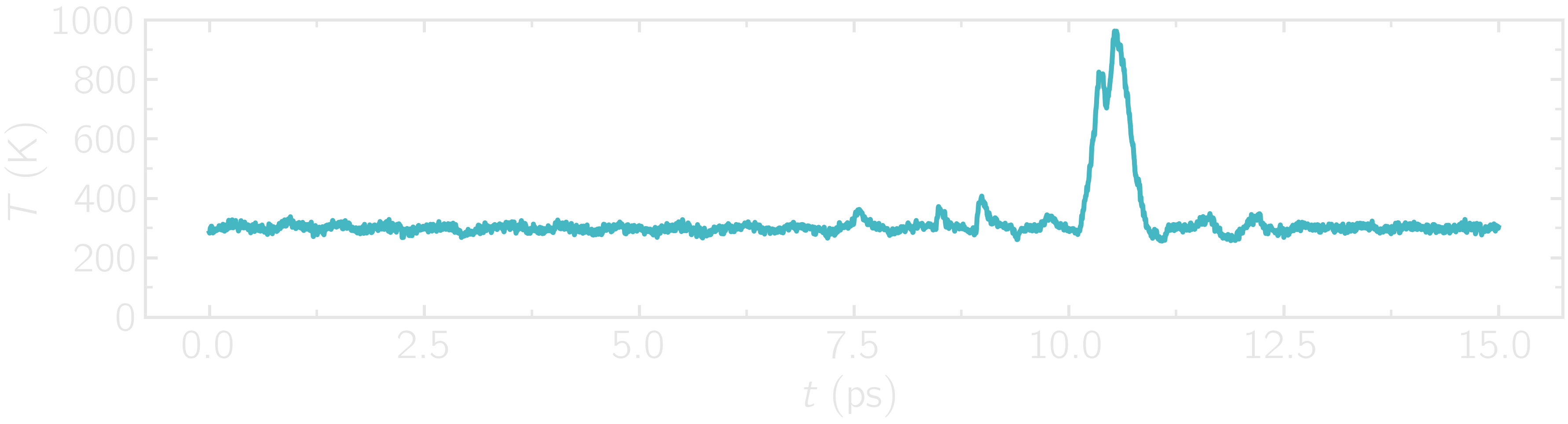
Figure: Evolution of the temperature \(T\) of the silica system over time \(t\). The material ruptures near \(t = 10~\text{ps}\).
At the end of the deformation, one can visualize the broken material using VMD. Notice the different charge values of the atoms located near the vacuum interfaces, compared to the atoms located in the bulk of the material.
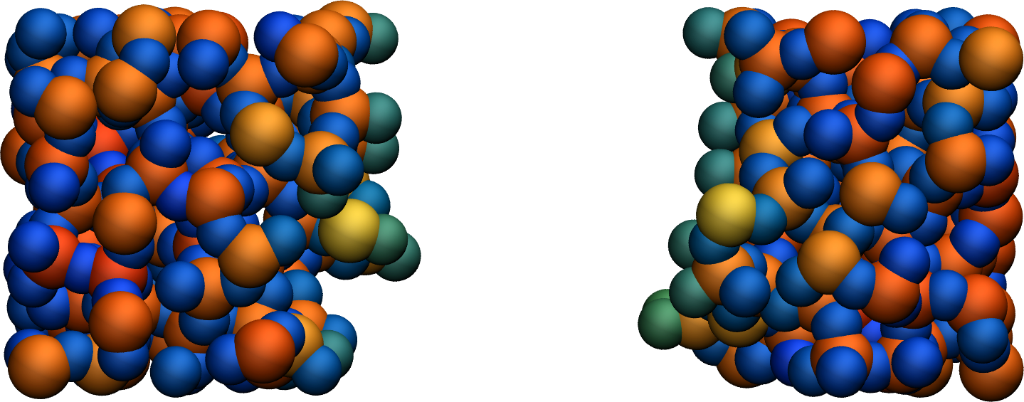
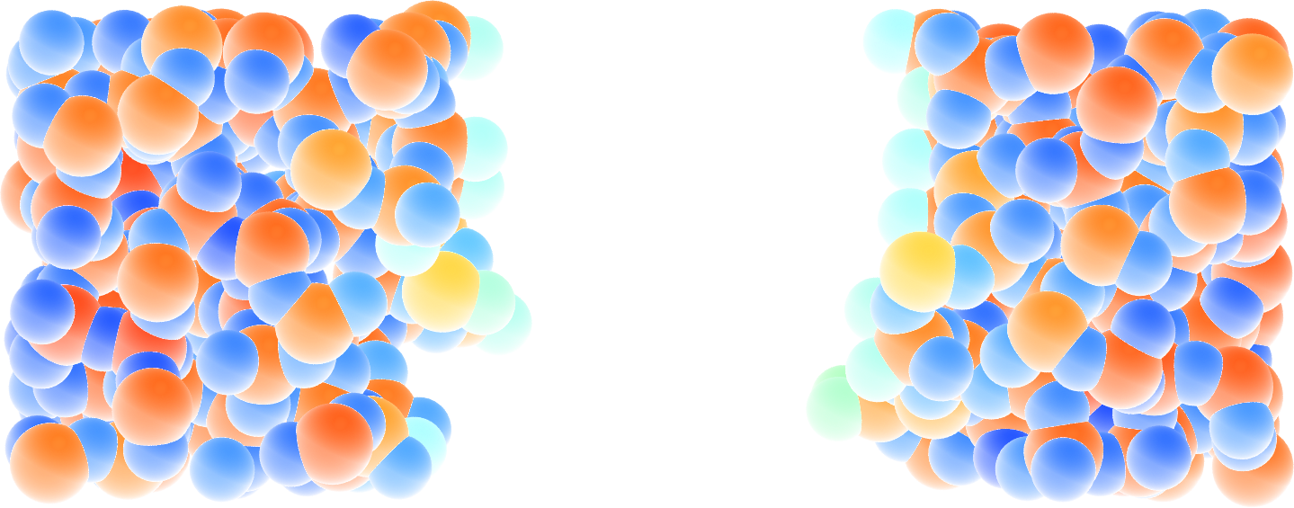
Figure: Amorphous silicon oxide after deformation. The atoms are colored by their charges. Dangling oxygen groups appear in greenish, bulk Si atoms with a charge of about \(1.8~\text{e}\) appear in red/orange, and bulk O atoms with a charge of about \(-0.9~\text{e}`\) appear in blue.
One can have a look at the charge distribution after deformation, as well as during the deformation.
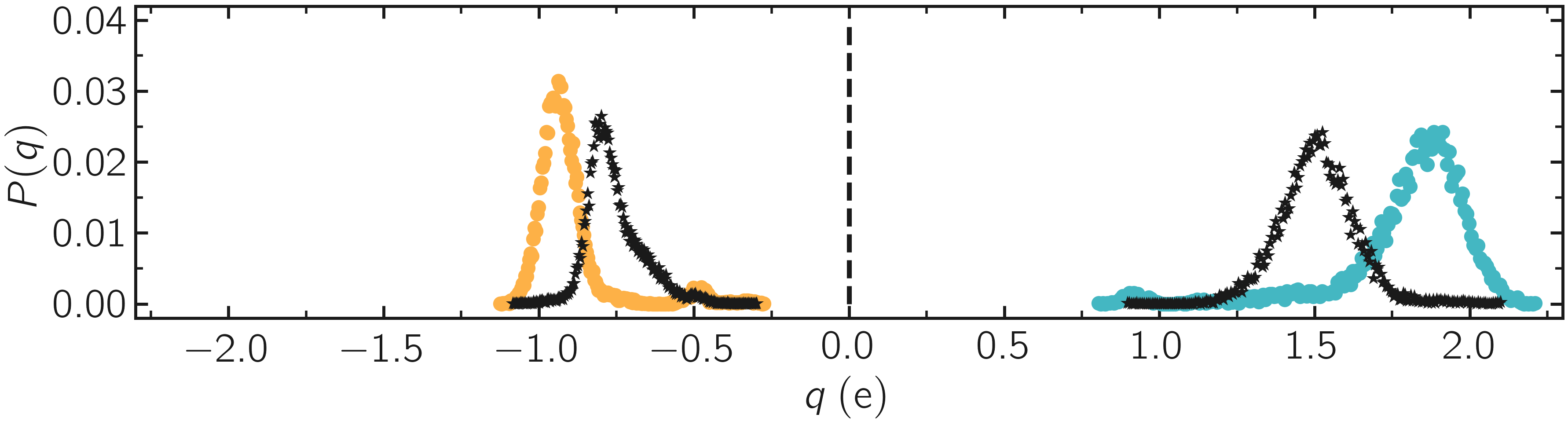
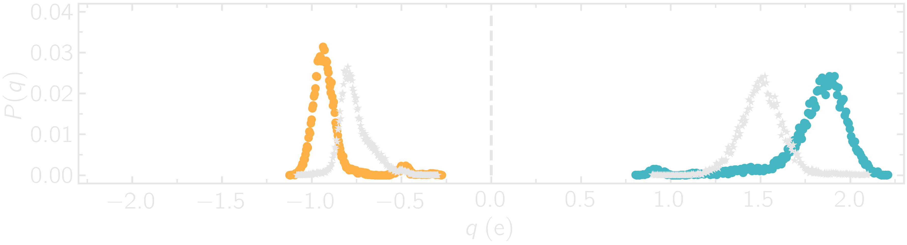
Figure: Distribution of charge of silicon (positive, blue) and oxygen (negative, orange) after deformation. The stars correspond to the charge distribution during deformation.
As expected, the final charge distribution slightly differs from the previously calculated. In my case, no new species were formed during the simulation, as can be seen from the species.log file:
#  Timestep    No_Moles    No_Specs   Si192O384
        5           1           1           1
(...)
#  Timestep    No_Moles    No_Specs   Si192O384
    30000           1           1           1
Sometimes, \(\text{O}_2\) molecules are formed during the deformation. If this is the case, the species.log file will look like:
#  Timestep    No_Moles    No_Specs   Si192O384
          5           1           1           1
(...)
#  Timestep    No_Moles    No_Specs   Si192O382          O2
      30000           1           1           1           1
Decorate the surface
In ambient conditions, some of the surface \(\text{SiO}_2\) atoms are chemically passivated by forming covalent bonds with hydrogen (H) atoms \(sulpizi2012silica\). Let us add hydrogen atoms randomly to the cracked silica and observe how the system evolves over time.
Next to RelaxSilica/ and Deform/, create a folder, and call it Decorate/. Then, let us modify the previously generated data file silica-deformed.data and make space for a third atom type. Copy silica-deformed.data from the Deform/ folder, and modify the first lines as follow:
576 atoms
3 atom types

-12.15958814509652 32.74516585669389 xlo xhi
2.316358282925984 18.26921942866687 ylo yhi
1.3959542953413138 19.189623416252907 zlo zhi

Masses

1 28.0855
2 15.999
3 1.008

(...)
Create a file named input.lammps into the Decorate/ folder, and copy the following lines into it:
units real
atom_style full

read_data silica-deformed.data
displace_atoms all move -12 0 0 # optional

pair_style reaxff NULL safezone 3.0 mincap 150
pair_coeff * * ../RelaxSilica/reaxCHOFe.ff Si O H
fix myqeq all qeq/reaxff 1 0.0 10.0 1.0e-6 reaxff maxiter 400
Here, the displace_atoms command was used to move the center of the crack near the center of the box. This step is optional but makes the visualization of the interface in VMD easier. A different value for the shift may be needed in your case, depending on the location of the crack.
A difference with the previous input is that three atom types are specified in the pair_coeff command, Si O H, instead of two.
Then, let us adapt some familiar commands to measure the charges of all three types of atoms, and output the charge values into log files:
group grpSi type 1
group grpO type 2
group grpH type 3
variable qSi equal charge(grpSi)/count(grpSi)
variable qO equal charge(grpO)/count(grpO)
variable qH equal charge(grpH)/(count(grpH)+1e-10)

thermo 5
thermo_style custom step temp etotal press vol &
    v_qSi v_qO v_qH
fix myspec all reaxff/species 5 1 5 species.log element Si O H
Here, the \(+1\text{e}-10\) was added to the denominator of the variable qH in order to avoid dividing by 0 at the beginning of the simulation.
Finally, let us create a loop with 10 steps, and create two hydrogen atoms at random locations at every step:
fix mynvt all nvt temp 300.0 300.0 100
timestep 0.5

label loop
variable a loop 10

variable seed equal 35672+${a}
create_atoms 3 random 2 ${seed} NULL overlap 2.6 maxtry 50
group grpH type 3
run 2000
write_dump all custom dump.${a}.lammpstrj id type q x y z

next a
jump SELF loop

write_data decorated.data
Here, a different lammpstrj file is created for each step of the loop to avoid creating dump files with varying numbers of atoms, which VMD can’t read.
Once the simulation is over, it can be seen from the species.log file that all the created hydrogen atoms reacted with the \(\text{SiO}_{2}\) structure to form surface groups (such as hydroxyl (-OH) groups).
# Timestep   No_Moles   No_Specs  Si192O384  H
  5          3          2         1          2
(...)
# Timestep   No_Moles No_Specs Si192O384H20
  20000      1        1        1
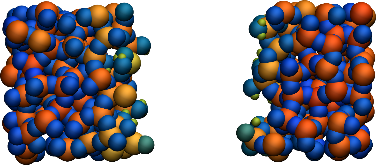
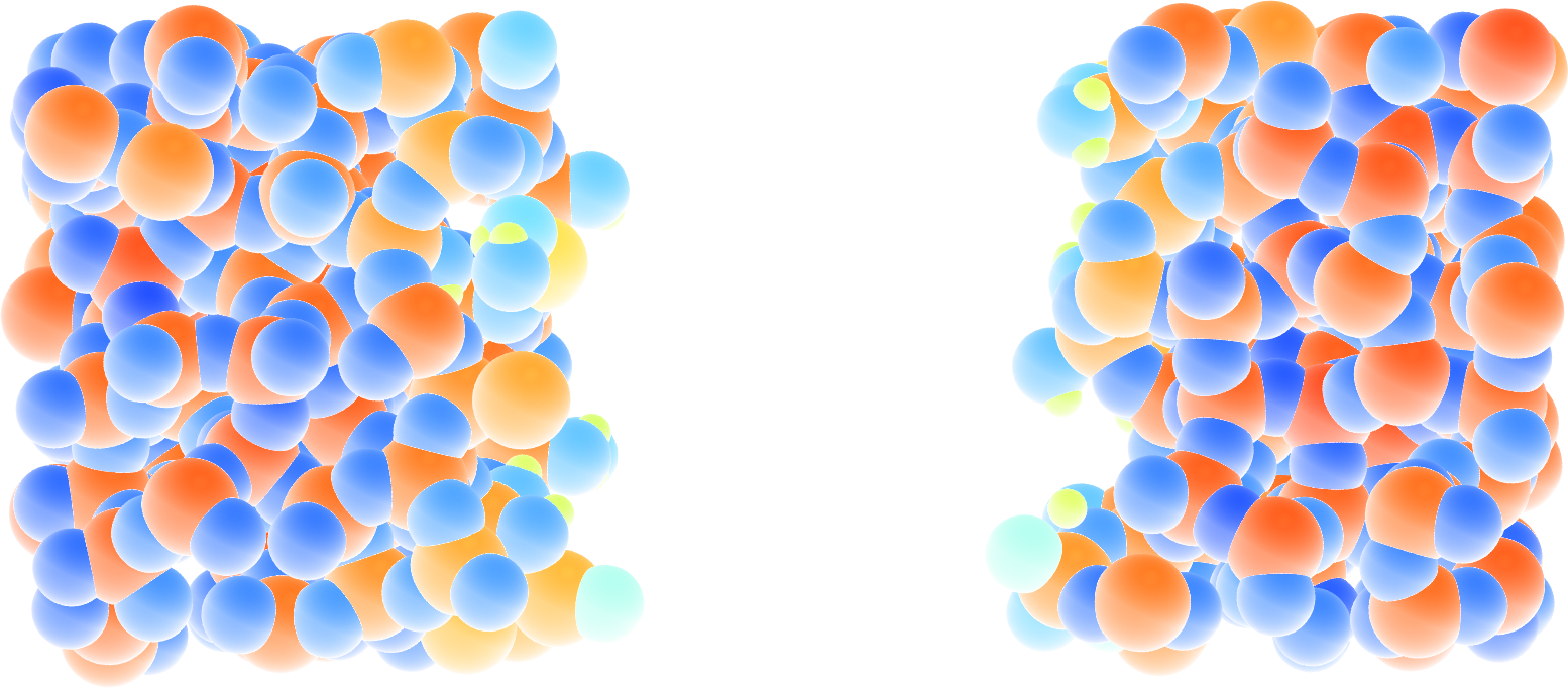
Figure: Cracked silicon oxide after the addition of hydrogen atoms. Some hydroxyl groups can be seen at the interfaces. The atoms are colored by their charges. Bulk Si atoms with a charge of about \(1.8~\text{e}\) appear in red/orange, and bulk O atoms with a charge of about \(-0.9 ~ \text{e}\) appear in blue.
You can access the input scripts and data files that are used in these tutorials from this Github repository. This repository also contains the full solutions to the exercises.
Going further with exercises
Each exercise comes with a proposed solution, see Solutions to the exercises.
Hydrate the structure
Add water molecules to the current structure, and follow the reactions over time.
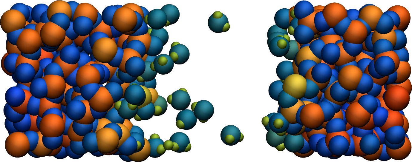
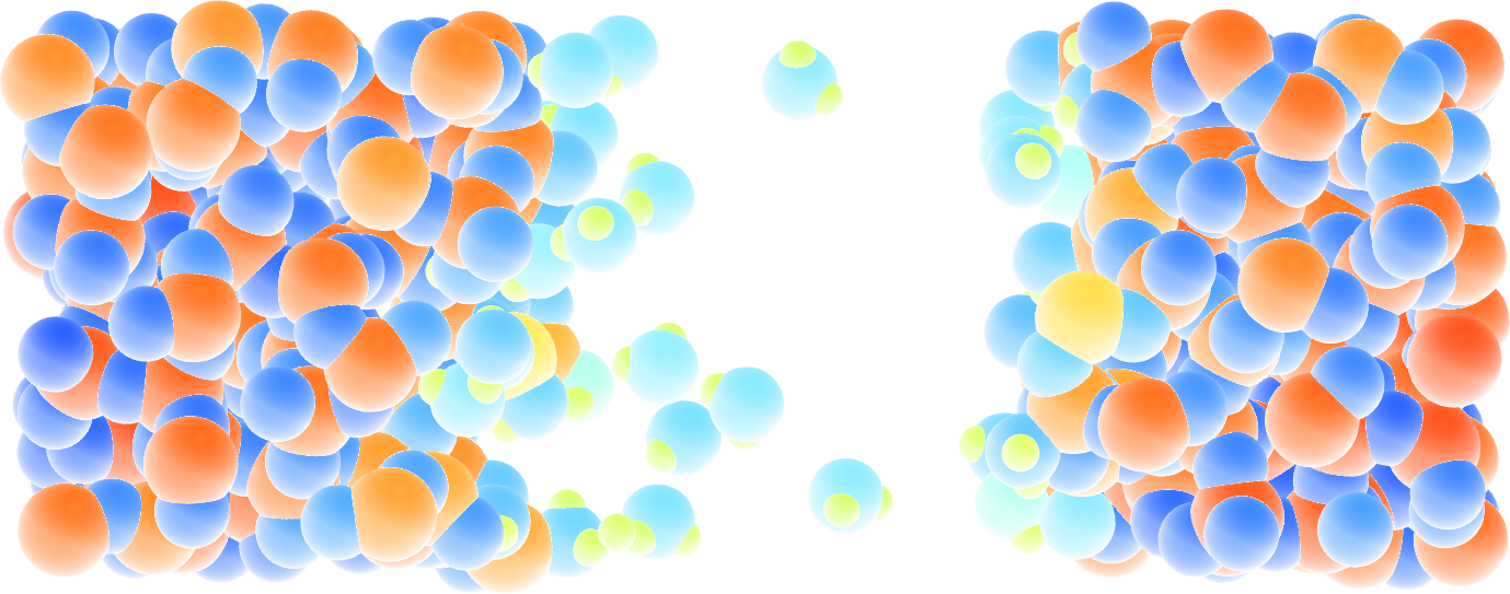
Figure: Cracked silicon oxide after the addition of water molecules. The atoms are colored by their charges.
A slightly acidic bulk solution
Create a bulk water system with a few hydronium ions (\(H_3O^+\) or \(H^+\)) using ReaxFF. The addition of hydronium ions will make the system acidic.
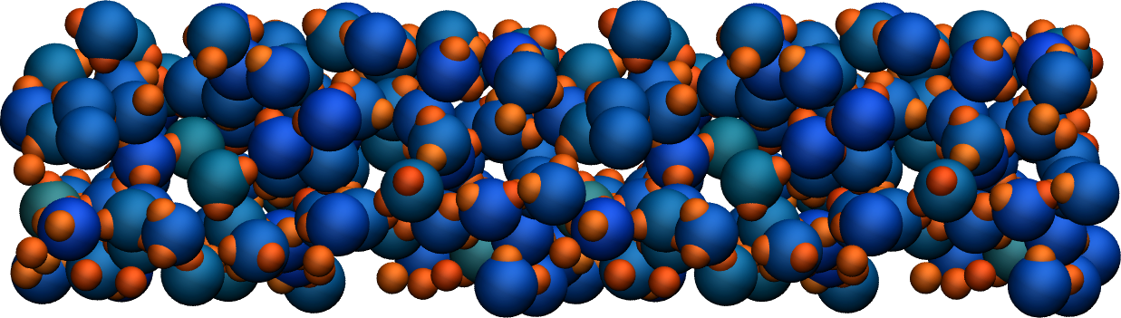
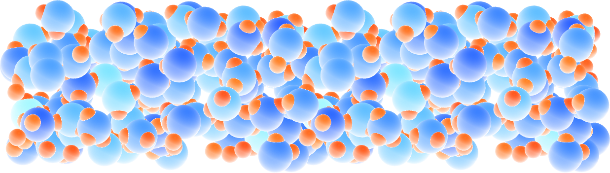
Figure: Slightly acidic bulk water simulated with ReaxFF. The atoms are colored by their charges.