Free energy calculation

Sampling a free energy barrier

The objective of this tutorial is to measure the free energy profile of particles through a barrier potential using two methods: free sampling and umbrella sampling [6, 7, 45]. To simplify the process and minimize computation time, the barrier potential will be imposed on the atoms using an additional force, mimicking the presence of a repulsive area in the middle of the simulation box without needing to simulate additional atoms. The procedure is valid for more complex systems and can be adapted to many other situations, such as measuring adsorption barriers near an interface or calculating translocation barriers through a membrane [46, 47, 48, 49, 50].

If you are completely new to LAMMPS, we recommend that you follow this tutorial on a simple Lennard-Jones fluid first.

Cite

If you find these tutorials useful, you can cite A Set of Tutorials for the LAMMPS Simulation Package by Simon Gravelle, Jacob R. Gissinger, and Axel Kohlmeyer (2025) [14]. You can access the full paper on arXiv.

This tutorial is compatible with the 29Aug2024 (update 2) LAMMPS version.

What is free energy

The free energy refers to the potential energy of a system that is available to perform work. In molecular simulations, it is common to calculate free energy differences between different states or conformations of a molecular system. This can be useful in understanding the thermodynamics of a system, predicting reaction pathways, and determining the stability of different molecular configurations.

Method 1: Free sampling

The most direct way to calculate a free energy profile is to extract the partition function from a classical (i.e. unbiased) molecular dynamics simulation, and then estimate the Gibbs free energy by using

(1)\[\Delta G = -RT \ln(p/p_0),\]

where \(\Delta G\) is the free energy difference, \(R\) is the gas constant, \(T\) is the temperature, \(p\) is the pressure, and \(p_0\) is a reference pressure. As an illustration, let us apply this method to a simple configuration that consists of a particles in a box in the presence of a position-dependent repulsive force that makes the center of the box a less favorable area to explore.

Basic LAMMPS parameters

To begin this tutorial, if you are using LAMMPS–GUI, select Start Tutorial 7 from the Tutorials menu and follow the instructions. Alternatively, if you are not using LAMMPS–GUI, create a new folder and add a file named free-energy.lmp. Open the file in a text editor and paste in the following content:

variable sigma equal 3.405
variable epsilon equal 0.238
variable U0 equal 1.5*${epsilon}
variable dlt equal 1.0
variable x0 equal 10.0

units real
atom_style atomic
pair_style lj/cut 3.822
pair_modify shift yes
boundary p p p

Here, we begin by defining variables for the Lennard-Jones interaction \(\sigma\) and \(\epsilon\) and for the repulsive potential \(U\), which are \(U_0\), \(\delta\), and \(x_0\) [see Eqs. (2)-(3) below]. The cut-off value of 3.822 Å was chosen to create a Weeks-Chandler-Andersen (WCA) potential, which is a truncated and purely repulsive LJ potential [51]. It was calculated as \(2^{1/6} \sigma\). The potential is also shifted to be equal to 0 at the cut-off using the pair_modify command.

System creation and settings

Let us define the simulation box and randomly add atoms by addying the following lines to free-energy.lmp:

region myreg block -50 50 -15 15 -50 50
create_box 1 myreg
create_atoms 1 random 200 34134 myreg overlap 3 maxtry 50

mass * 39.95
pair_coeff * * ${epsilon} ${sigma}

The variables \(U_0\), \(\delta\), and \(x_0\), defined in the previous subsection, are used here to create the repulsive potential, restricting the atoms from exploring the center of the box:

(2)\[U = U_0 \left[ \arctan \left( \dfrac{x+x_0}{\delta} \right) - \arctan \left(\dfrac{x-x_0}{\delta} \right) \right].\]

Taking the derivative of the potential with respect to \(x\), we obtain the expression for the force that will be imposed on the atoms:

(3)\[F = \dfrac{U_0}{\delta} \left[ \dfrac{1}{(x-x_0)^2/\delta^2+1} - \dfrac{1}{(x+x_0)^2/\delta^2+1} \right].\]

The figure below shows the potential \(U\) and force \(F\) along the \(x\)-axis. With \(U_0 = 1.5 \epsilon = 0.36\,\text{kcal/mol},\) \(U_0\) is of the same order of magnitude as the thermal energy \(k_\text{B} T = 0.24\,\text{kcal/mol}\), where \(k_\text{B} = 0.002\,\text{kcal/mol/K}\) is the Boltzmann constant and \(T = 119.8\,\text{K}\) is the temperature used in this simulation. Under these conditions, particles are expected to frequently overcome the energy barrier due to thermal agitation.

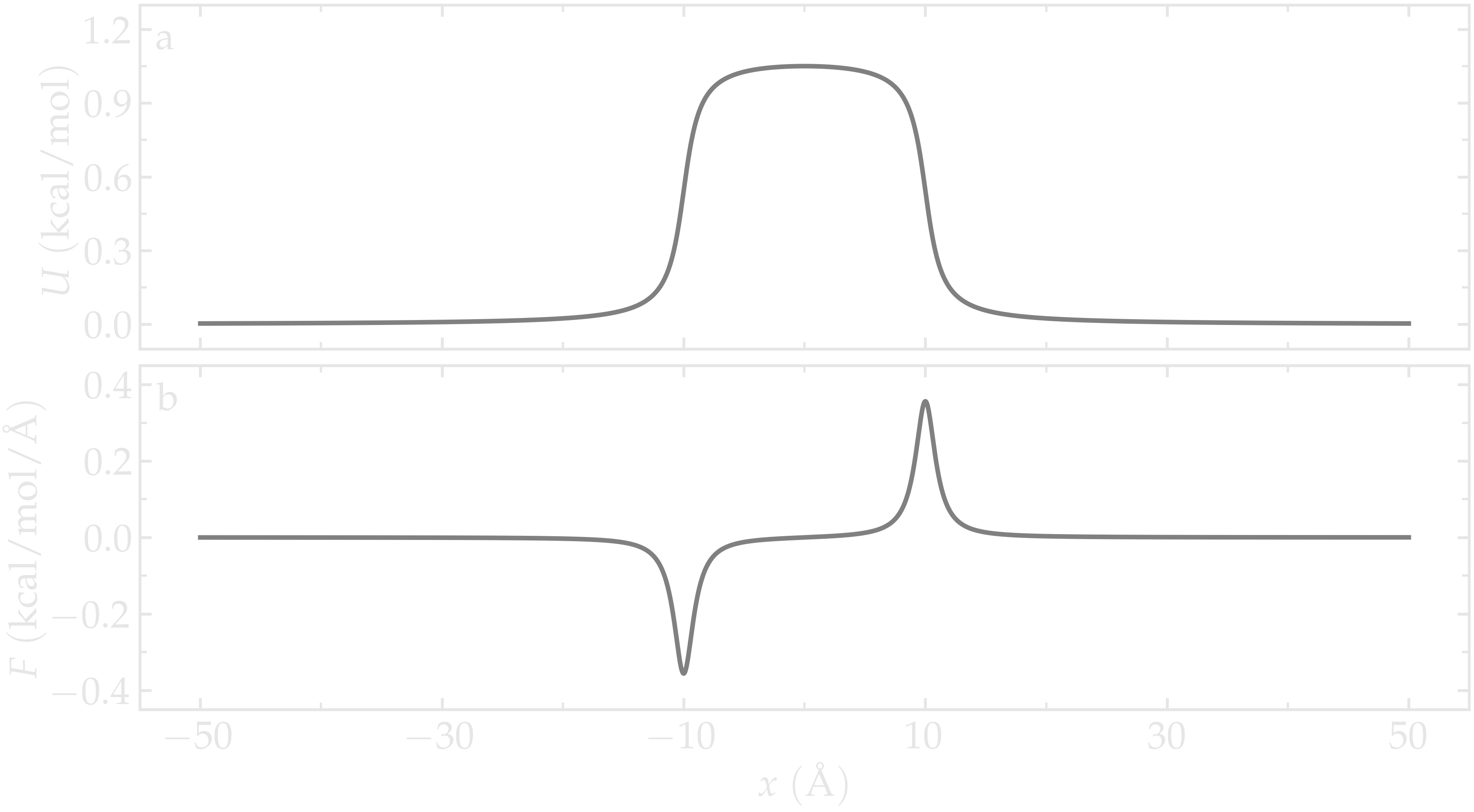
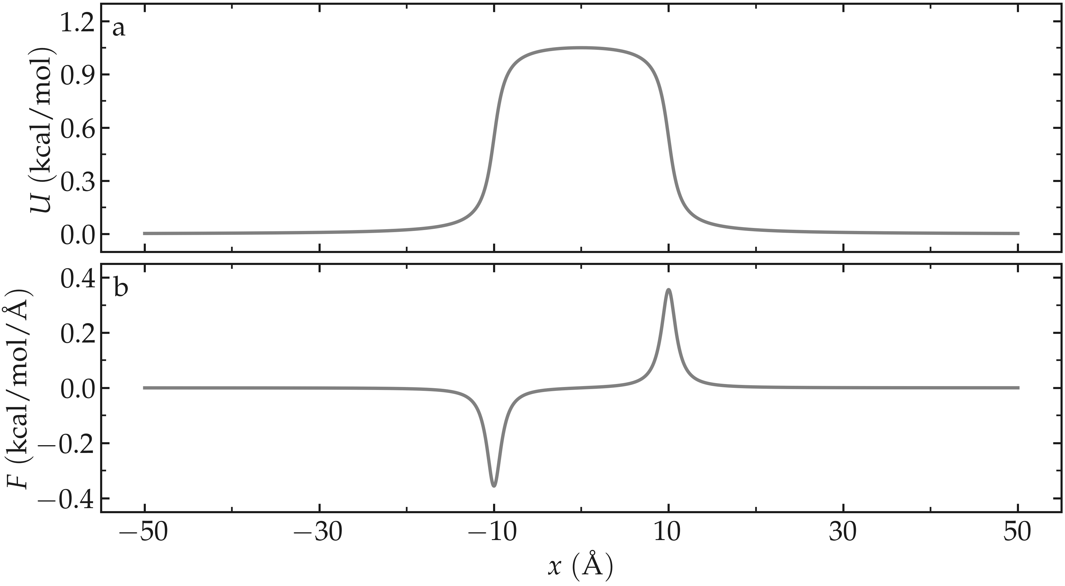
Figure: Potential \(U\) given in Eq. (2) (a) and force \(F\) given in Eq. (3) (b) as functions of the coordinate \(x\). Here, \(U_0 = 0.36~\text{kcal/mol}\), \(\delta = 1.0~\text{Å}\), and \(x_0 = 10~\text{Å}\).

We impose the force \(F(x)\) to the atoms in the simulation using the fix addforce command. Add the following lines to free-energy.lmp:

variable U atom ${U0}*atan((x+${x0})/${dlt})-${U0}*atan((x-${x0})/${dlt})
variable F atom ${U0}/((x-${x0})^2/${dlt}^2+1)/${dlt}-${U0}/((x+${x0})^2/${dlt}^2+1)/${dlt}
fix myadf all addforce v_F 0.0 0.0 energy v_U

Next, we combine the fix nve with a fix langevin thermostat:

fix mynve all nve
fix mylgv all langevin 119.8 119.8 500 30917

When combining these two commands, the MD simulation operates in the NVT ensemble, maintaining a constant number of atoms \(N\), constant volume \(V\), and a temperature \(T\) that fluctuates around a target value.

To ensure that the equilibration time is sufficient, we will track the evolution of the number of atoms in the central - energetically unfavorable - region, referred to as mymes, using the n_center variable:

region mymes block -${x0} ${x0} INF INF INF INF
variable n_center equal count(all,mymes)
thermo_style custom step temp etotal v_n_center
thermo 10000

For visualization, use one of the following options: the dump image command to create .ppm images of the system, or the dump atom command to write a VMD-compatible trajectory to a file:

# Option 1
dump viz1 all image 50000 myimage-*.ppm type type shiny 0.1 box yes 0.01 view 180 90 zoom 6 size 1600 500 fsaa yes
dump_modify viz1 backcolor white acolor 1 cyan adiam 1 3 boxcolor black

# Option 2
dump viz2 all atom 50000 free-energy.lammpstrj

Finally, let us perform an equilibration of 50000 steps, using a timestep of \(2\,\text{fs}\), corresponding to a total duration of \(100\,\text{ps}\):

timestep 2.0
run 50000

Run the simulation with LAMMPS. The number of atoms in the central region, \(n_\mathrm{center}\), reaches its equilibrium value after approximately \(40\,\text{ps}\).

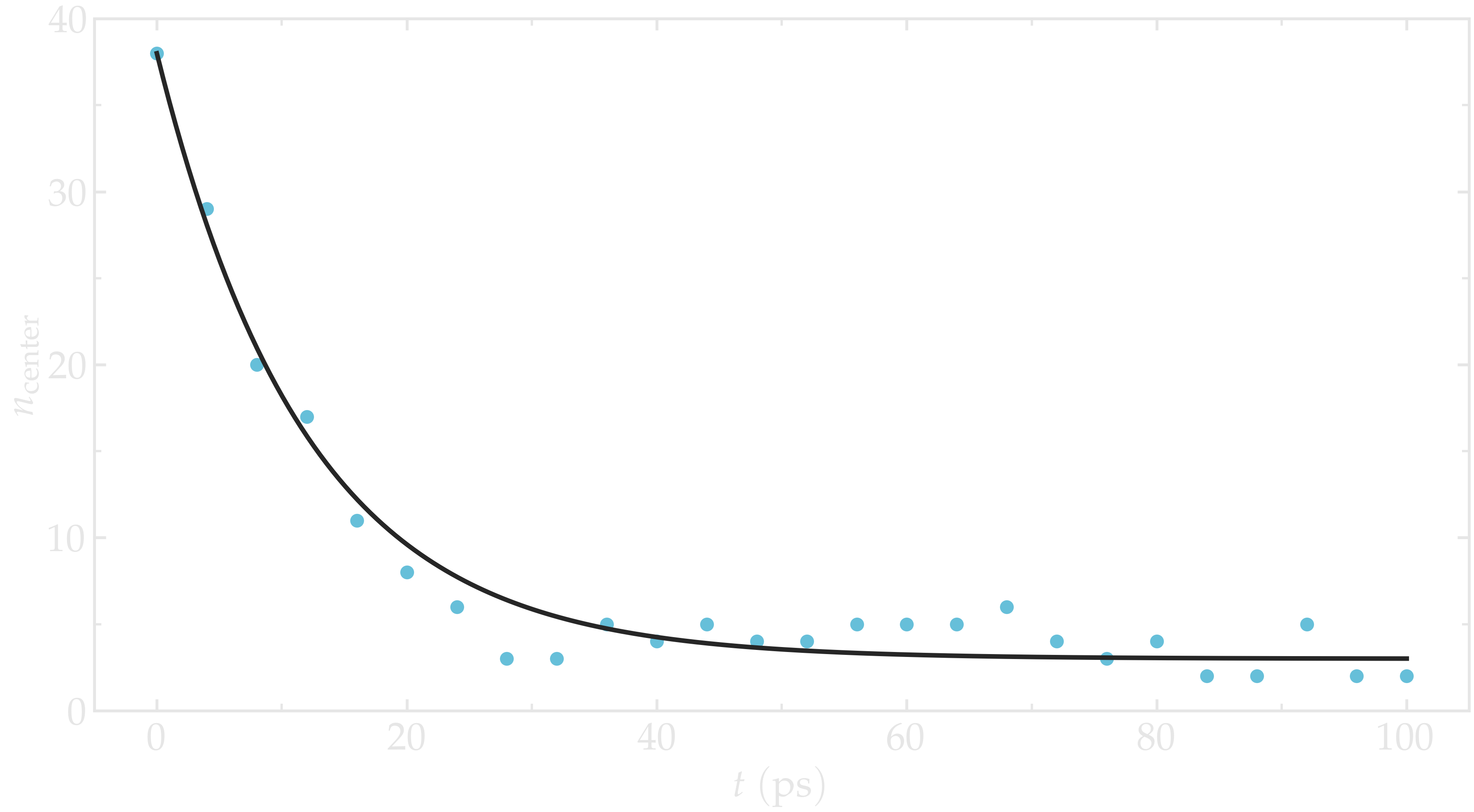
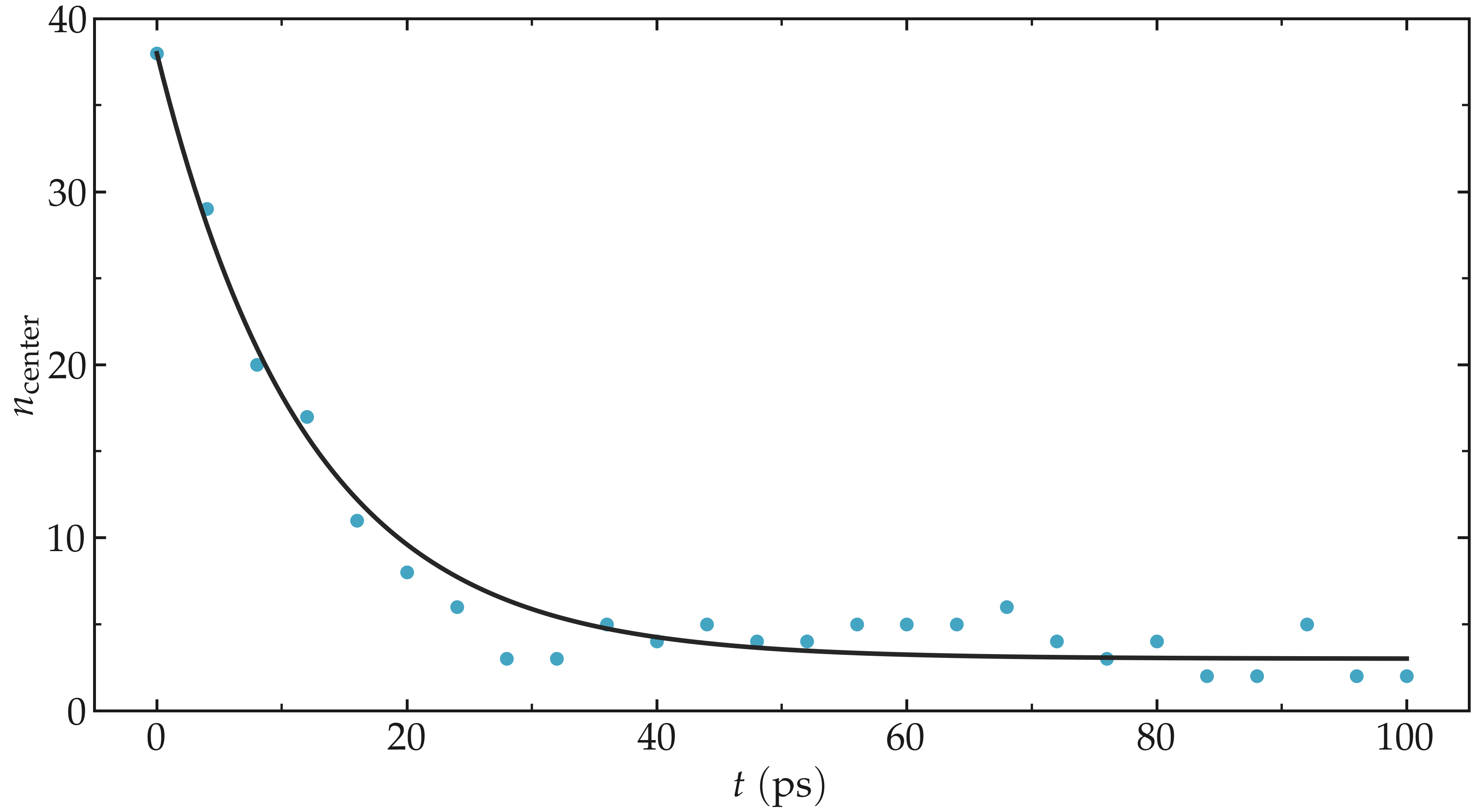
Figure: Evolution of the number of atoms \(n_\text{center}\) in the central region mymes as a function of time \(t\) during equilibration. The dark line is \(n_\text{center} = 22 \exp(-t/160)+5\) and serves as a guide for the eyes. Here, \(U_0 = 0.36~\text{kcal/mol}\), \(\delta = 1.0~\text{Å}\), and \(x_0 = 10~\text{Å}\).

Run and data acquisition

Once the system is equilibrated, we will record the density profile of the atoms along the \(x\)-axis using the ave/chunk command. Add the following line to free-energy.lmp:

reset_timestep 0

thermo 200000

compute cc1 all chunk/atom bin/1d x 0.0 2.0
fix myac all ave/chunk 100 20000 2000000 cc1 density/number file free-sampling.dat

run 2000000

The step count is reset to 0 using reset_timestep to synchronize it with the output times of fix density/number. Run the simulation using LAMMPS.

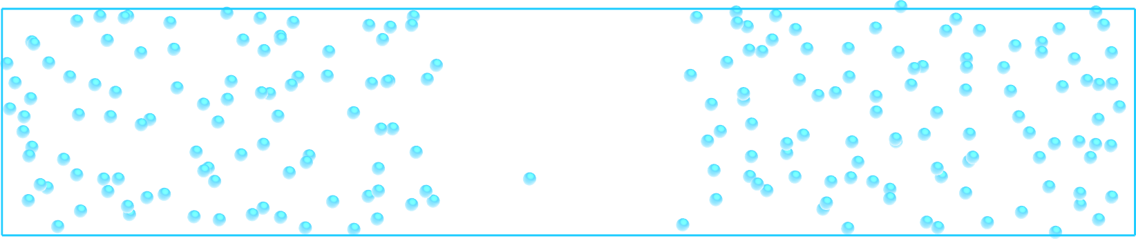
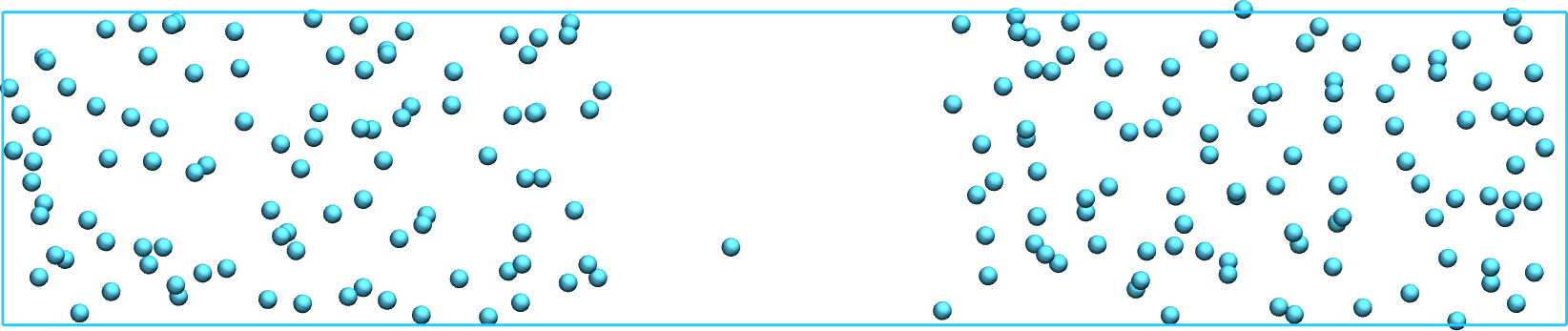
Figure: Snapshot of the system simulated during the free sampling step of the tutorial. The atoms density is the lowest in the central part of the box, mymes. Here, \(U_0 = 0.36~\text{kcal/mol}\), \(\delta = 1.0~\text{Å}\), and \(x_0 = 10~\text{Å}\).

Data analysis

Once the simulation is complete, the density profile from free-sampling.dat shows that the density in the center of the box is about two orders of magnitude lower than inside the reservoir. Next, we plot \(-R T \ln(\rho/\rho_\mathrm{bulk})\) (i.e. Eq. (1) where the pressure ratio \(p/p_\mathrm{bulk}\) is replaced by the density ratio \(\rho/\rho_\mathrm{bulk}\), assuming the system behaves as an ideal gas) and compare it with the imposed potential \(U\) from Eq. (2). The reference density, \(\rho_\text{bulk} = 0.0009~\text{Å}^{-3}\), was estimated by measuring the density of the reservoir from the raw density profiles. The agreement between the MD results and the imposed energy profile is excellent, despite some noise in the central part, where fewer data points are available due to the repulsive potential.

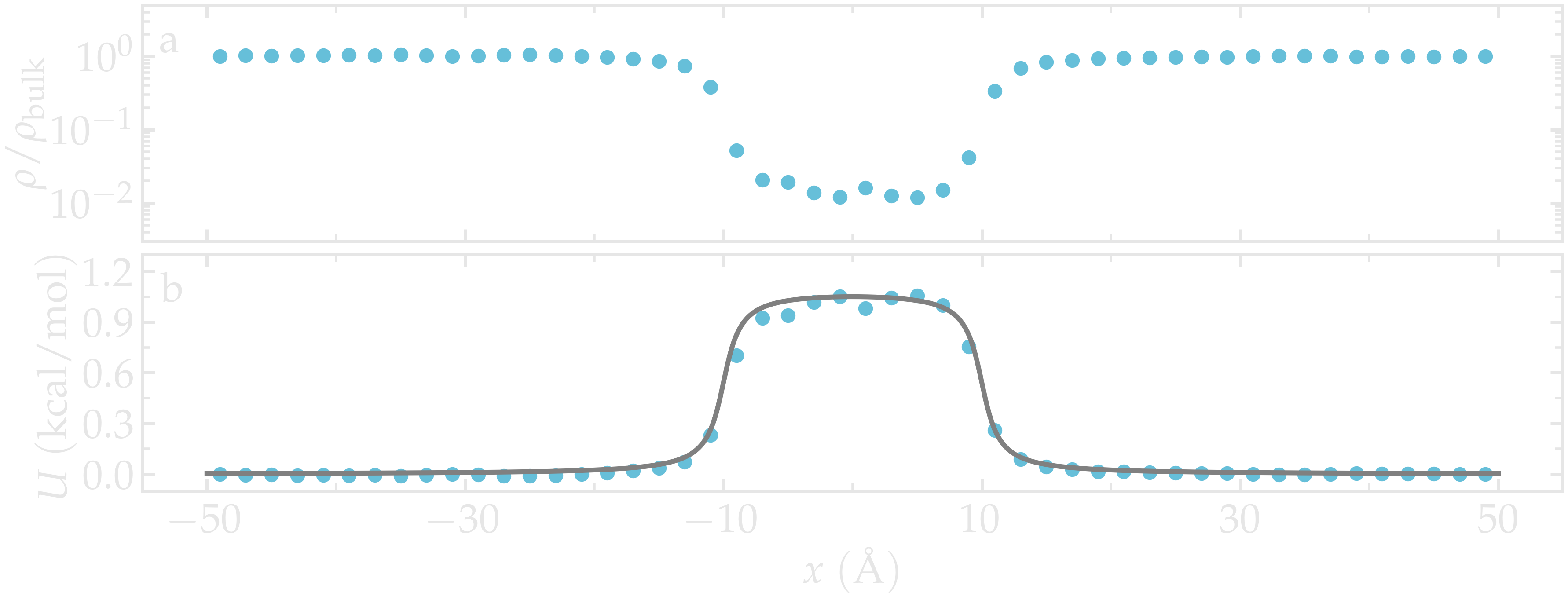
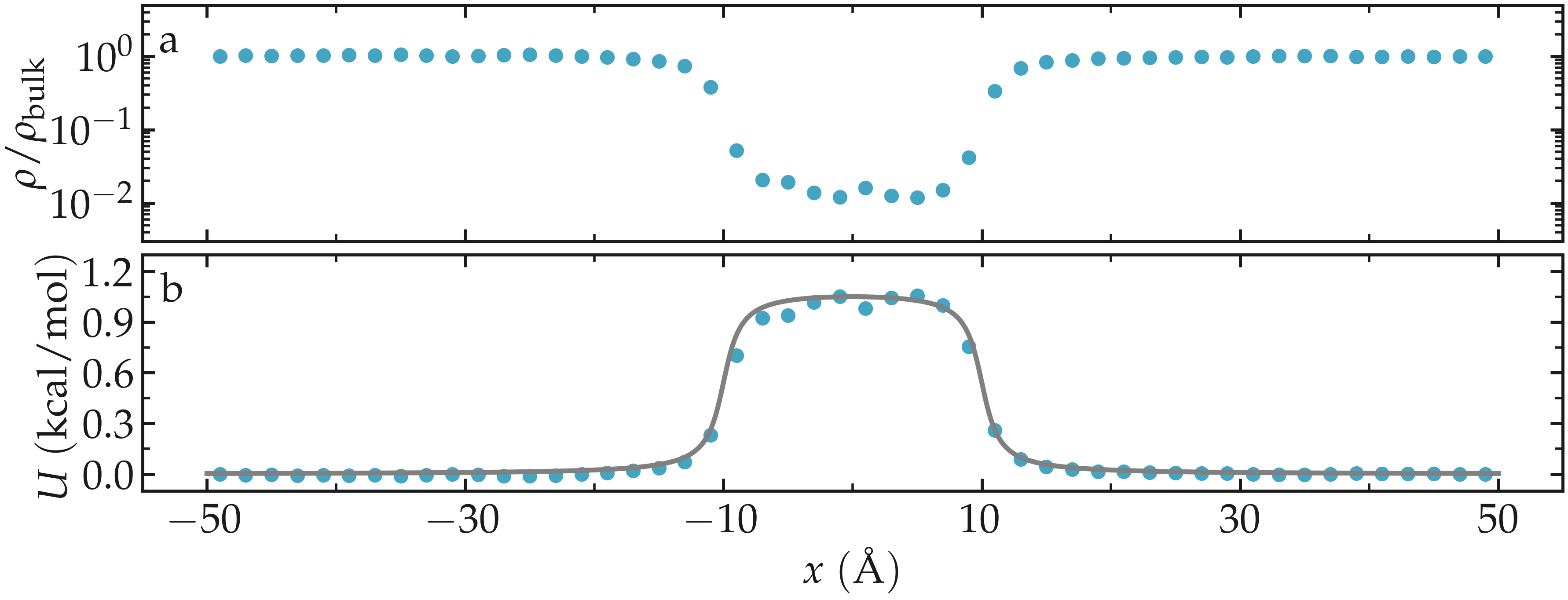
Figure: a) Fluid density, \(\rho\), along the \(x\) direction. b) Potential, \(U\), as a function of \(x\) measured using free sampling (disks) compared to the imposed potential given in Eq. (2) (line). Here, \(U_0 = 0.36~\text{kcal/mol}\), \(\delta = 1.0~\text{Å}\), \(x_0 = 10~\text{Å}\), and the measured reference density in the reservoir is \(\rho_\text{bulk} = 0.0009~\text{Å}^{-3}\).

The limits of free sampling

Increasing the value of \(U_0\) reduces the average number of atoms in the central region, making it difficult to achieve a high-resolution free energy profile. For example, running the same simulation with \(U_0 = 10 \epsilon\), corresponding to \(U_0 \approx 10 k_\text{B} T\), results in no atoms exploring the central part of the simulation box during the simulation. In such a case, employing an enhanced sampling method is recommended, as done in the next section.

Method 2: Umbrella sampling

Umbrella sampling is a biased molecular dynamics method in which additional forces are added to a chosen atom to force it to explore the more unfavorable areas of the system [6, 7, 45]. Here, to encourage one of the atoms to explore the central region of the box, we apply a potential \(V\) and force it to move along the \(x\)-axis. The chosen path is called the axis of reaction. Several simulations (called windows) will be conducted with varying positions for the center of the applied biasing. The results will be analyzed using the weighted histogram analysis method (WHAM) [52, 53], which allows for the removal of the biasing effect and ultimately deduces the unbiased free energy profile.

LAMMPS input script

If you are using LAMMPS–GUI, open the file named free-energy.lmp. Alternatively, if you are not using LAMMPS–GUI, create a new input file and paste in the following content:

variable sigma equal 3.405
variable epsilon equal 0.238
variable U0 equal 10*${epsilon}
variable dlt equal 1.0
variable x0 equal 10
variable k equal 0.5

units real
atom_style atomic
pair_style lj/cut 3.822
pair_modify shift yes
boundary p p p

The first difference from the previous case is the larger value for the repulsive potential \(U_0\), which makes the central area of the system very unlikely to be visited by free particles. The second difference is the introduction of the variable \(k\), which will be used for the biasing potential.

Let us create a simulation box with two atom types, including a single particle of type 2, by adding the following lines to umbrella-sampling.lmp:

region myreg block -50 50 -15 15 -50 50
create_box 2 myreg
create_atoms 2 single 0 0 0
create_atoms 1 random 199 34134 myreg overlap 3 maxtry 50

Next, we assign the same mass and LJ parameters to both atom types 1 and 2, and place the atoms of type 2 into a group named topull:

mass * 39.948
pair_coeff * * ${epsilon} ${sigma}
group topull type 2

Then, the same potential \(U\) and force \(F\) are applied to all the atoms, together with the same fix nve and fix langevin commands:

variable U atom ${U0}*atan((x+${x0})/${dlt})-${U0}*atan((x-${x0})/${dlt})
variable F atom ${U0}/((x-${x0})^2/${dlt}^2+1)/${dlt}-${U0}/((x+${x0})^2/${dlt}^2+1)/${dlt}
fix myadf all addforce v_F 0.0 0.0 energy v_U

fix mynve all nve
fix mylgv all langevin 119.8 119.8 500 30917

Next, we perform a brief equilibration to prepare for the umbrella sampling run:

thermo 5000

# Option 1
dump viz1 all image 50000 myimage-*.ppm type type shiny 0.1 box yes 0.01 view 180 90 zoom 6 size 1600 500 fsaa yes
dump_modify viz1 backcolor white acolor 1 cyan acolor 2 red adiam 1 3 adiam 2 3 boxcolor black

# Option 2
dump viz2 all atom 50000 free-energy.lammpstrj

timestep 2.0
run 50000

So far, our code resembles that of Method 1, except for the additional particle of type 2. Particles of types 1 and 2 are identical, with the same mass and LJ parameters. However, the particle of type 2 will also be exposed to the biasing potential \(V\), which forces it to explore the central part of the box.

Now, we create a loop with 15 steps and progressively move the center of the bias potential by increments of 0.4 nm. Add the following lines to umbrella-sampling.lmp:

variable a loop 25
label loop

variable xdes equal 4*${a}-32
variable xave equal xcm(topull,x)
fix mytth topull spring tether ${k} ${xdes} 0 0 0

run 20000

fix myat1 all ave/time 10 10 100 v_xave v_xdes file umbrella-sampling.${a}.dat

run 200000
unfix myat1
next a
jump SELF loop

The spring command imposes the additional harmonic potential \(V\) with the previously defined spring constant \(k\). The center of the harmonic potential, \(x_\text{des}\), successively takes values from \(-28\,\text{Å}\) to \(28\,\text{Å}\). For each value of \(x_\text{des}\), an equilibration step of 40 ps is performed, followed by a step of 400 ps during which the position of the particle of type 2 along the \(x\)-axis, \(x_\text{ave}\), is saved in data files named umbrella-sampling.i.dat, where \(i\) ranges from 1 to 15. Run the umbrella-sampling.lmp file using LAMMPS.

Note

The value of \(k\) should be chosen with care: if \(k\) is too small the particle won’t follow the biasing potential, and if \(k\) is too large there will be no overlapping between the different windows, leading to poor reconstruction of the free energy profile. See the section Side note: On the choice of k.

WHAM algorithm

To generate the free energy profile from the particle positions saved in the umbrella-sampling.i.dat files, we use the WHAM [52, 53] algorithm as implemented by Alan Grossfield [54]. You can download it from Alan Grossfield’s website. Make sure you download the WHAM code version 2.1.0 or later which introduces the units command-line option used below. The executable called wham generated by following the instructions from the website must be placed next to umbrella-sampling.lmp. To apply the WHAM algorithm to our simulation, we need a metadata file containing:

• the paths to all the data files,

• the values of \(x_\text{des}\),

• the values of \(k\).

Download the umbrella-sampling.meta file and save it next to umbrella-sampling.lmp. Then, run the WHAM algorithm by typing the following command in the terminal:

./wham units real -30 30 50 1e-8 119.8 0 umbrella-sampling.meta umbrella-sampling.dat

where -30 and 30 are the boundaries, 50 is the number of bins, 1e-8 is the tolerance, and 119.8 is the temperature in Kelvin. A file called umbrella-sampling.dat is created, containing the free energy profile in kcal/mol. The resulting PMF can be compared with the imposed potential \(U\), showing excellent agreement.

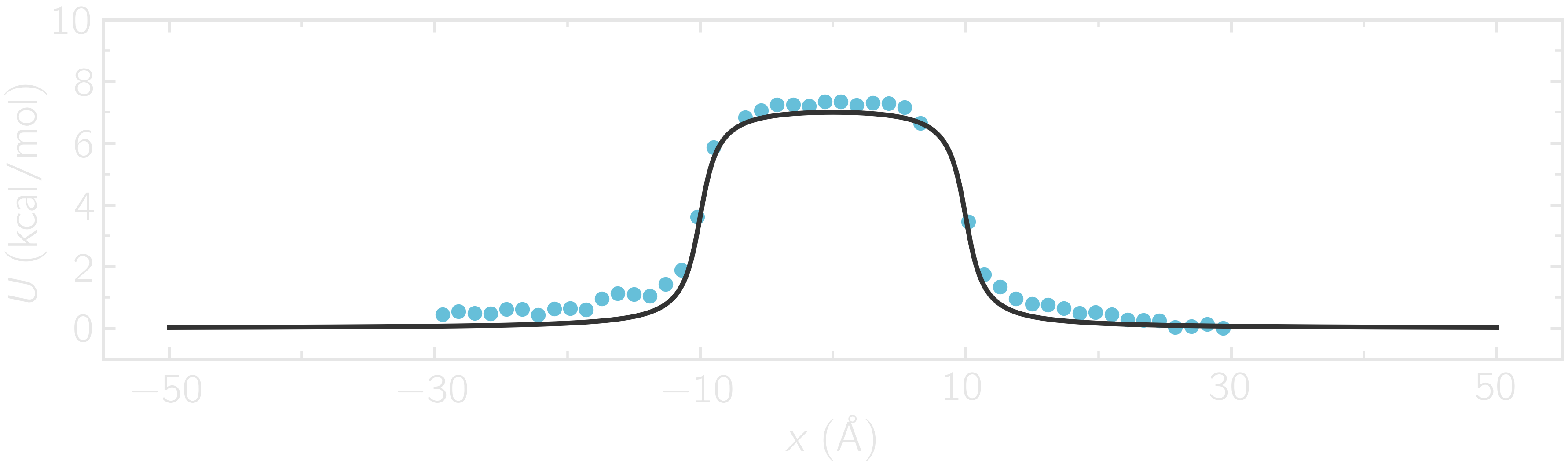
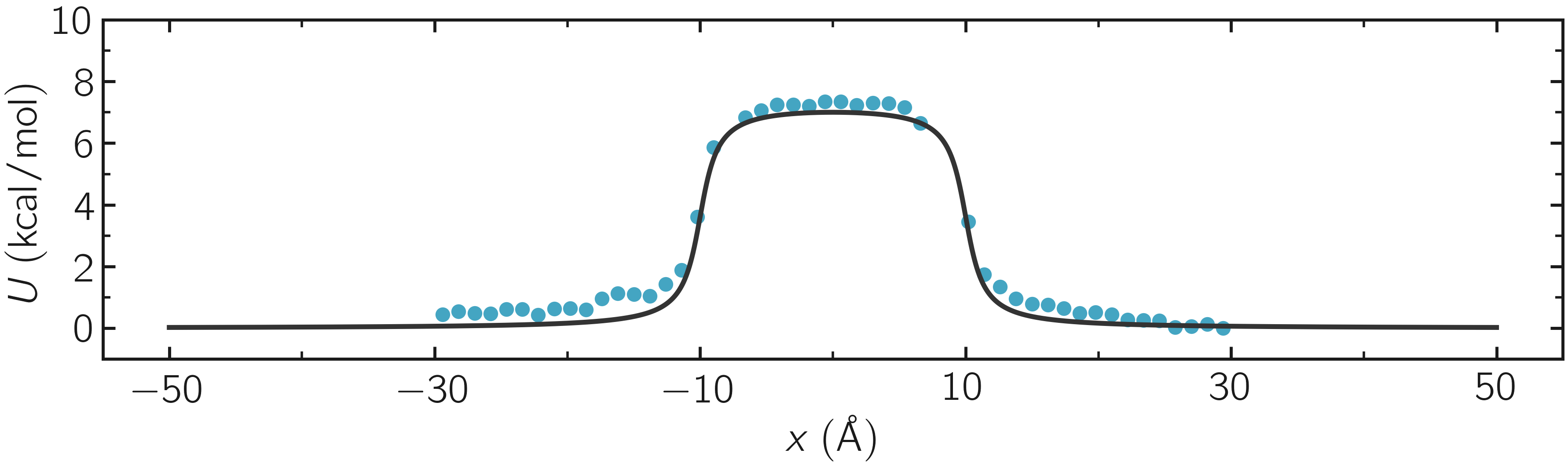
Figure: The potential, \(U\), as a function of \(x\), measured using umbrella sampling (disks), is compared to the imposed potential given in Eq. (2) (line). Parameters are \(U_0 = 2.38~\text{kcal/mol}\), \(\delta = 1.0~\text{Å}\), and \(x_0 = 10~\text{Å}\).

Remarkably, this excellent agreement is achieved despite the very short calculation time and the high value for the energy barrier. Achieving similar results through free sampling would require performing extremely long and computationally expensive simulations.

Side note: On the choice of \(k\)

One difficult part of umbrella sampling is choosing the value of \(k\). Ideally, you want the biasing potential to be strong enough to force the chosen atom or molecule to move along the chosen axis, while also allowing fluctuations in its position large enough to ensure some overlap in the probability density between neighboring positions. Here, as an illustration, three different values of \(k\) are tested:

• If \(k\) is too small, the biasing potential is too weak to force the particle to explore the region of interest, making it impossible to reconstruct the PMF (see panel a in the figure below).

• If \(k\) is “appropriate”, the particle explores the entire axis, and the probability distributions are strongly impacted by the potential one wants to probe, as shown in panel b.

• If \(k\) is too large, the biasing potential dominates over the potential one wants to probe, which reduces the sensitivity of the method (panel c).

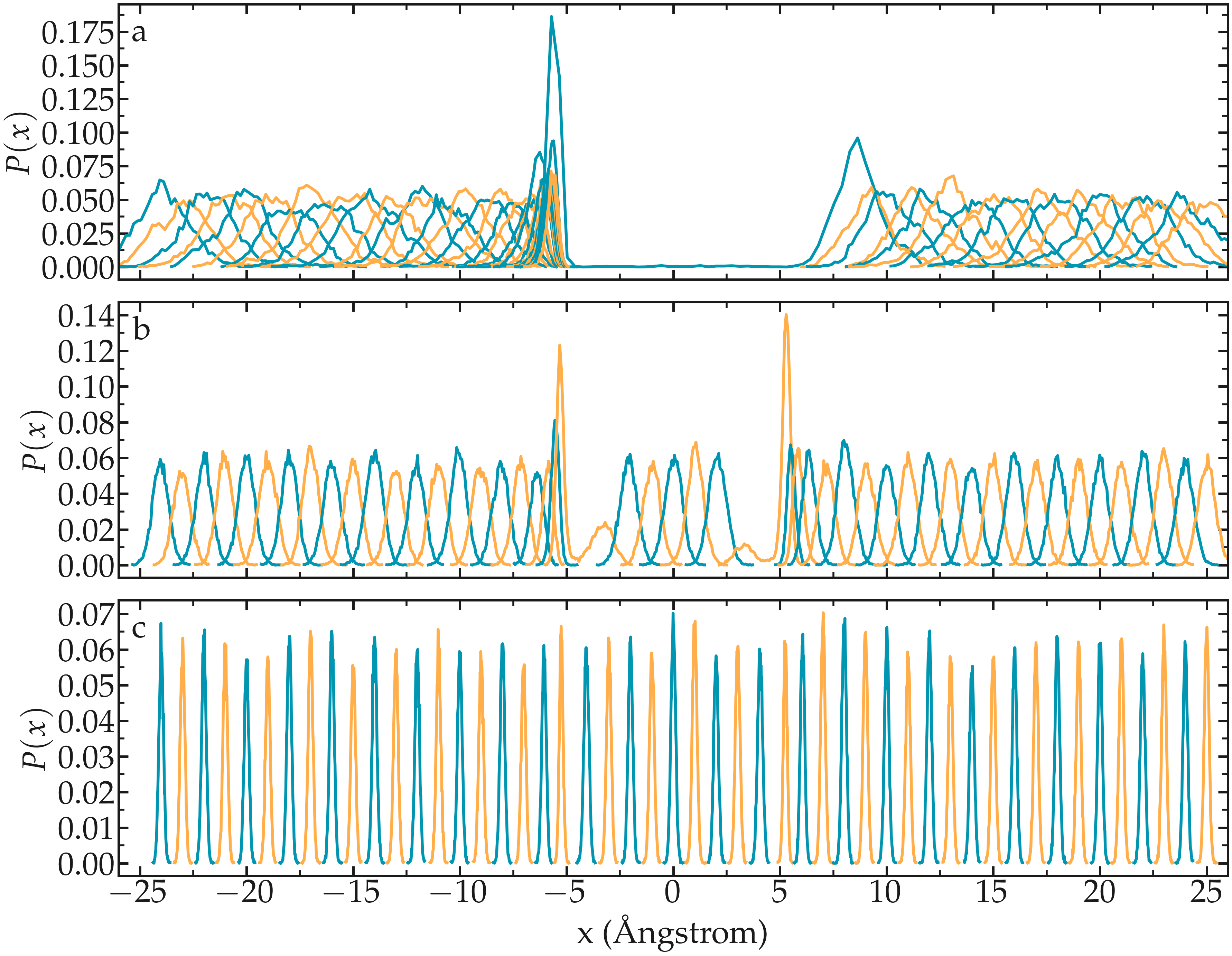
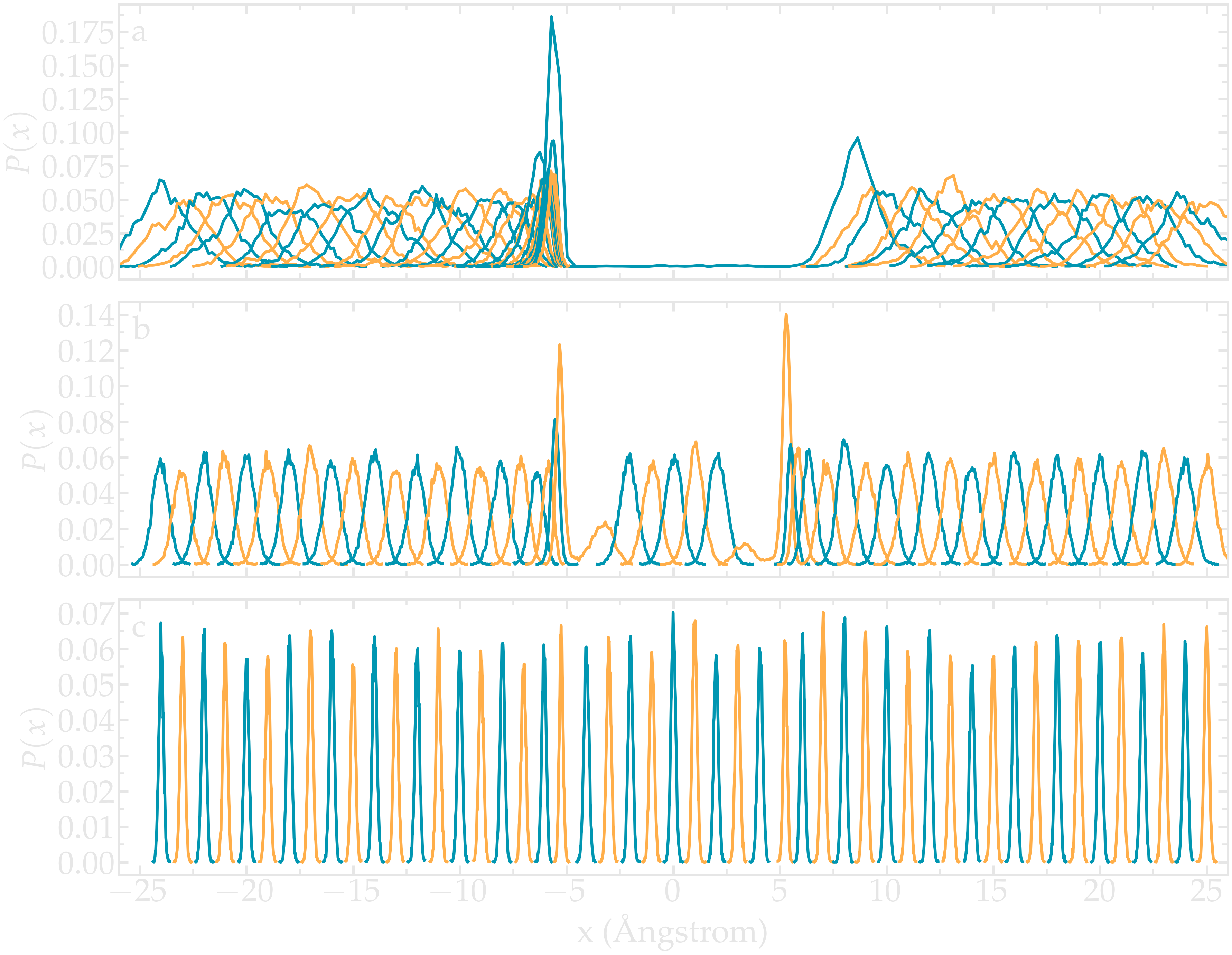
Figure: Probability density for each run with \(k = 0.15\,\text{kcal}/\text{mol}/\mathrm{Å}^2\) (a) (a value that is too small to bring the particle into the central region), \(k = 1.5\,\text{kcal}/\text{mol}/\mathrm{Å}^2\) (b) (a value that allows the particle to explore the entire path), and \(k = 15\,\text{kcal}/\text{mol}/\mathrm{Å}^2\) (c) (a value so strong that it becomes difficult to perceive the effect of the probed potential).

Cite

You can access the input scripts and data files that are used in these tutorials from a dedicated Github repository. This repository also contains the full solutions to the exercises.

Going further with exercises

The binary fluid that won’t mix

1 - Create the system

Create a molecular simulation with two species of respective types 1 and 2. Apply different potentials \(U1\) and \(U2\) on particles of types 1 and 2, respectively, so that particles of type 1 are excluded from the center of the box, while at the same time particles of type 2 are excluded from the rest of the box.

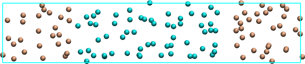
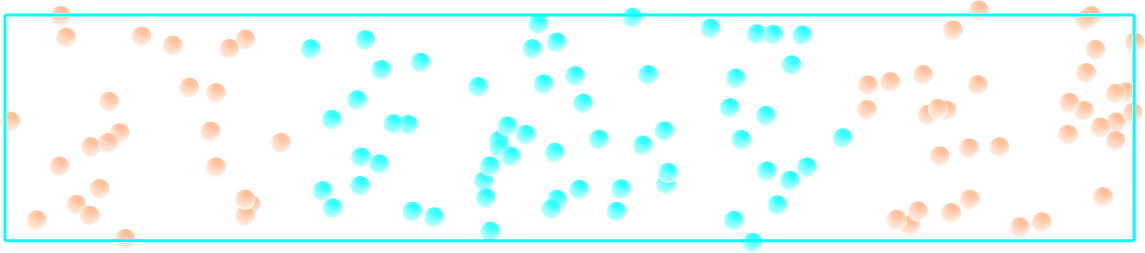
Figure: Particles of type 1 and 2 separated by two different potentials.

2 - Measure the PMFs

Using the same protocol as the one used in the tutorial (i.e. umbrella sampling with the wham algorithm), extract the PMF for each particle type.

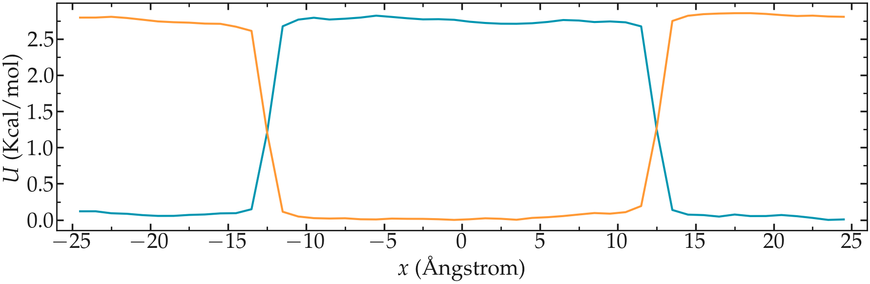
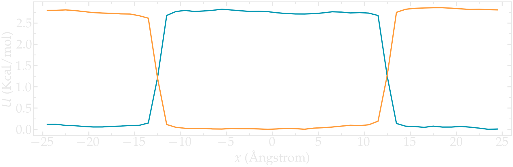
Figure: PMFs calculated for both atom types.

Particles under convection

Use a similar simulation as the one from the tutorial, with a repulsive potential in the center of the box. Add force to the particles and force them to flow in the \(x\) direction.

Re-measure the potential in the presence of the flow, and observe the difference with the reference case in the absence of flow.

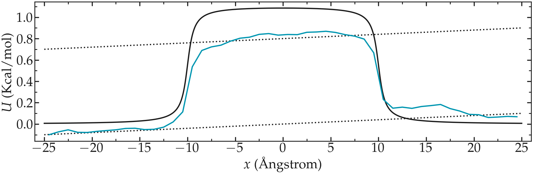
Figure: PMF calculated in the presence of a net force that is inducing the convection of the particles from left to right.

Surface adsorption of a molecule

Apply umbrella sampling to calculate the free energy profile of ethanol in the direction normal to a crystal solid surface (here made of sodium chloride). Find the topology files and parameter file.

Use the following lines for starting the input.lammps:

units real # style of units (A, fs, Kcal/mol)
atom_style full # molecular + charge
bond_style harmonic
angle_style harmonic
dihedral_style harmonic
boundary p p p # periodic boundary conditions
pair_style lj/cut/coul/long 10 # cut-off 1 nm
kspace_style pppm 1.0e-4
pair_modify mix arithmetic tail yes

The PMF normal to a solid wall serves to indicate the free energy of adsorption, which can be calculated from the difference between the PMF far from the surface, and the PMF at the wall.

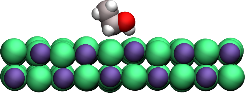
Figure: A single ethanol molecule next to a crystal NaCl(100) wall.

The PMF shows a minimum near the solid surface, which indicates a good affinity between the wall and the molecule.

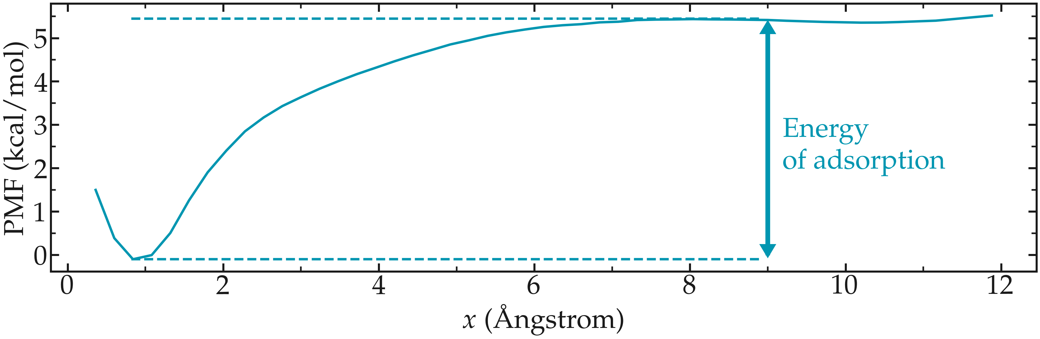
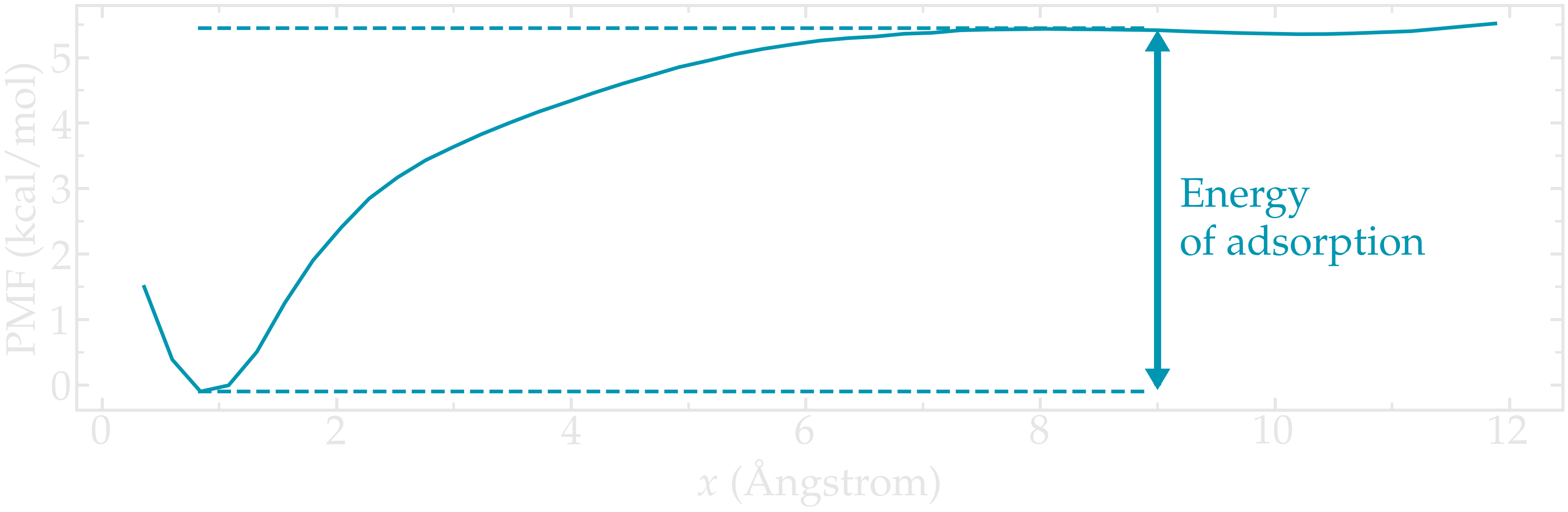
Figure: PMF for a single ethanol molecule next to a NaCl solid surface. The position of the wall is in \(x=0\). The arrow highlights the difference between the energy of the molecule when adsorbed to the solid surface, and the energy far from the surface. This difference corresponds to the free energy of adsorption.

Alternatively to using ethanol, feel free to download the molecule of your choice, for instance from the Automated Topology Builder (ATB). Make your life simpler by choosing a small molecule like CO2.