Lennard-Jones fluid

The very basics of LAMMPS through a simple example

The objective of this tutorial is to perform simple MD simulations using LAMMPS. The system consists of a Lennard-Jones fluid composed of neutral particles with two different effective diameters, contained within a cubic box with periodic boundary conditions. In this tutorial, basic MD simulations in the microcanonical (NVE) and canonical (NVT) ensembles are performed, and basic quantities are calculated, including the potential and kinetic energies.

This tutorial is compatible with the 29Aug2024 (update 2) LAMMPS version.

Cite

If you find these tutorials useful, you can cite A Set of Tutorials for the LAMMPS Simulation Package by Simon Gravelle, Jacob R. Gissinger, and Axel Kohlmeyer (2025) [14]. You can access the full paper on arXiv.

My first input

To run a simulation using LAMMPS, you need to write an input script containing a series of commands for LAMMPS to execute, similar to Python or Bash scripts. For clarity, the input scripts for this tutorial will be divided into five categories, which will be filled out step by step. To set up this tutorial using LAMMPS graphical user interface (LAMMPS–GUI), select Start LAMMPS Tutorial 1 from the Tutorials menu and follow the instructions. This will select (or create, if needed) a folder, place the initial input file initial.lmp in it, and open the file in the LAMMPS–GUI Editor window:

# PART A - ENERGY MINIMIZATION
# 1) Initialization
# 2) System definition
# 3) Settings
# 4) Visualization
# 5) Run

If you are not using LAMMPS-GUI

All tutorials can be followed without using LAMMPS-GUI. To do so, create a new folder and add a file named initial.lmp inside it. Open the file in a text editor of your choice and copy the previous lines into it.

Everything that appears after a hash symbol (#) is a comment and ignored by LAMMPS. These five categories are not required in every input script an do not necessarily need to be in that exact order. For instance, the Settings and the Visualization categories could be inverted, or the Visualization category could be omitted. However, note that LAMMPS reads input files from top to bottom and processes each command immediately. Therefore, the Initialization and System definition categories must appear at the top of the input, and the Run category must appear at the bottom. Also, the specifics of some commands can change after global settings are modified, so the order of commands in the input script is important.

Initialization

In the first section of the script, called Initialization, global parameters for the simulation are defined, such as units, boundary conditions (e.g., periodic or non-periodic), and atom types (e.g., uncharged point particles or extended spheres with a radius and angular velocities). These commands must be executed before creating the simulation box or they will cause an error. Similarly, many LAMMPS commands may only be entered after the simulation box is defined. Only a limited number of commands may be used in both cases. Update the initial.lmp file so that the Initialization section appears as follows:

# 1) Initialization
units lj
dimension 3
atom_style atomic
boundary p p p

The first line, units lj, specifies the use of reduced units, where all quantities are dimensionless. This unit system is a popular choice for simulations that explore general statistical mechanical principles, as it emphasizes relative differences between parameters rather than representing any specific material. The second line, dimension 3, specifies that the simulation is conducted in 3D space, as opposed to 2D, where atoms are confined to move only in the xy-plane. The third line, atom_style atomic, designates the atomic style for representing simple, individual point particles. In this style, each particle is treated as a point with a mass, making it the most basic atom style. Other atom styles can incorporate additional attributes for atoms, such as charges, bonds, or molecule IDs, depending on the requirements of the simulated model. The last line, boundary p p p, indicates that periodic boundary conditions are applied along all three directions of space, where the three p stand for \(x\), \(y\), and \(z\), respectively. Alternatives are fixed non-periodic (f), shrink-wrapped non-periodic (s), and shrink-wrapped non-periodic with minimum (m). For non-periodic boundaries, different options can be assigned to each dimension, making configurations like boundary p p fm valid for systems such as slab geometries.

Note

Strictly speaking, none of the four commands specified in the Initialization section are mandatory, as they correspond to the default settings for their respective global properties. However, explicitly specifying these defaults is considered good practice to avoid confusion when sharing input files with other LAMMPS users.

Each LAMMPS command is accompanied by extensive online documentation that details the different options for that command. From the LAMMPS–GUI editor buffer, you can access the documentation by right-clicking on a line containing a command (e.g., units lj) and selecting View Documentation for `units'. This action should prompt your web browser to open the corresponding URL for the online manual.

The next step is to create the simulation box and populate it with atoms. Modify the System definition category of initial.lmp as shown below:

# 2) System definition
region simbox block -20 20 -20 20 -20 20
create_box 2 simbox
create_atoms 1 random 1500 34134 simbox overlap 0.3
create_atoms 2 random 100 12756 simbox overlap 0.3

The first line, region simbox (...), defines a region named simbox that is a block (i.e., a rectangular cuboid) extending from -20 to 20 units along all three spatial dimensions. The second line, create_box 2 simbox, initializes a simulation box based on the region simbox and reserves space for two types of atoms.

Note

From this point on, any command referencing an atom type larger than 2 will trigger an error. While it is possible to allocate more atom types than needed, you must assign a mass and provide force field parameters for each atom type. Failing to do so will cause LAMMPS to terminate with an error.

The third line, create_atoms (...), generates 1500 atoms of type 1 at random positions within the simbox region. The integer 34134 is a seed for the internal random number generator, which can be changed to produce different sequences of random numbers and, consequently, different initial atom positions. The fourth line adds 100 atoms of type 2. Both create_atoms commands use the optional argument overlap 0.3, which enforces a minimum distance of 0.3 units between the randomly placed atoms. This constraint helps avoid close contacts between atoms, which can lead to excessively large forces and simulation instability.

Settings

Next, we specify the settings for the two atom types. Modify the Settings category of initial.lmp as follows:

# 3) Settings
mass 1 1.0
mass 2 5.0
pair_style lj/cut 4.0
pair_coeff 1 1 1.0 1.0
pair_coeff 2 2 0.5 3.0

The two mass commands assign a mass of 1.0 and 5.0 units to the atoms of type 1 and 2, respectively. The third line, pair_style lj/cut 4.0, specifies that the atoms will be interacting through a Lennard-Jones (LJ) potential with a cut-off equal to \(r_c = 4.0\) length units [15, 16]:

(1)\[E_{ij}(r) = 4 \epsilon_{ij} \left[ \left( \dfrac{\sigma_{ij}}{r} \right)^{12} - \left( \dfrac{\sigma_{ij}}{r} \right)^{6} \right], \quad \text{for} \quad r < r_c,\]

where \(r\) is the inter-particle distance, \(\epsilon_{ij}\) is the depth of the potential well that determines the interaction strength, and \(\sigma_{ij}\) is the distance at which the potential energy equals zero. The indexes \(i\) and \(j\) refer to pairs of particle types. The fourth line, pair_coeff 1 1 1.0 1.0, specifies the Lennard-Jones coefficients for interactions between pairs of atoms of type 1: the energy parameter \(\epsilon_{11} = 1.0\) and the distance parameter \(\sigma_{11} = 1.0\). Similarly, the last line sets the Lennard-Jones coefficients for interactions between atoms of type 2, \(\epsilon_{22} = 0.5\), and \(\sigma_{22} = 3.0\).

Note

By default, LAMMPS calculates the cross coefficients for different atom types using geometric average: \(\epsilon_{ij} = \sqrt{\epsilon_{ii} \epsilon_{jj}}\), \(\sigma_{ij} = \sqrt{\sigma_{ii} \sigma_{jj}}\). In the present case, \(\epsilon_{12} = \sqrt{1.0 \times 0.5} = 0.707\), and \(\sigma_{12} = \sqrt{1.0 \times 3.0} = 1.732\).

Single-point energy

The system is now fully parameterized, and the input is ready to compute forces. Let us complete the two remaining categories, Visualization and Run, by adding the following lines to initial.lmp:

# 4) Visualization
thermo 10
thermo_style custom step etotal press
# 5) Run
run 0 post no

The thermo 10 command instructs LAMMPS to print thermodynamic information to the console every specified number of steps, in this case, every 10 simulation steps. The thermo_style custom command defines the specific outputs, which in this case are the step number (step), total energy \(E\) (etotal), and pressure \(p\) (press). The run 0 post no command instructs LAMMPS to initialize forces and energy without actually running the simulation. The post no option disables the post-run summary and statistics output.

You can now run LAMMPS (basic commands for running LAMMPS are provided in Running LAMMPS. The simulation should finish quickly.

With the default settings, LAMMPS–GUI will open two windows: one displaying the console output and another with a chart. The Output window will display information from the executed commands, including the total energy and pressure at step 0, as specified by the thermodynamic data request. Since no actual simulation steps were performed, the Charts window will be empty.

Snapshot image – At this point, you can create a snapshot image of the current system using the Image Viewer window, which can be accessed by clicking the Create Image button in the Run menu. The image viewer works by instructing LAMMPS to render an image of the current system using its internal rendering library via the dump image command. The resulting image is then displayed, with various buttons available to adjust the view and rendering style. This will always capture the current state of the system.

Energy minimization

Now, replace the run 0 post no command line with the following minimize command:

# 5) Run
minimize 1.0e-6 1.0e-6 1000 10000

This tells LAMMPS to perform an energy minimization of the system. Specifically, LAMMPS will compute the forces on all atoms and then update their positions according to a selected algorithm, aiming to reduce the potential energy. By default, LAMMPS uses the conjugate gradient (CG) algorithm [17]. The simulation will stop as soon as the minimizer algorithm cannot find a way to lower the potential energy. Note that, except for trivial systems, minimization algorithms will find a local minimum rather than the global minimum.

Run the minimization and observe that LAMMPS-GUI captures the output and updates the chart in real time. This run executes quickly (depending on your computer’s capabilities), but LAMMPS-GUI may fail to capture some of the thermodynamic data. In that case, use the Preferences dialog to reduce the data update interval and switch to single-threaded, unaccelerated execution in the Accelerators tab. You can repeat the run; each new attempt will start fresh, resetting the system and re-executing the script from the beginning.

Run the minimization. The potential energy, \(U\), decreases from a positive value to a negative value (as can also be seen in the figure below). Note that during energy minimization, the potential energy equals the total energy of the system, \(E = U\), since the kinetic energy, \(K\), is zero. The initially positive potential energy is expected, as the atoms are created at random positions within the simulation box, with some in very close proximity to each other. This proximity results in a large initial potential energy due to the repulsive branch of the Lennard-Jones potential [i.e., the term in \(1/r^{12}\) in Eq. (1)]. As the energy minimization progresses, the energy decreases - first rapidly - then more gradually, before plateauing at a negative value. This indicates that the atoms have moved to reasonable distances from one another.

Create and save a snapshot image of the simulation state after the minimization, and compare it to the initial image. You should observe that the atoms are clumping together as they move toward positions of lower potential energy.

Molecular dynamics

After energy minimization, any overlapping atoms are displaced, and the system is ready for a molecular dynamics simulation. To continue from the result of the minimization step, append the MD simulation commands to the same input script, initial.lmp. Add the following lines immediately after the minimize command:

# PART B - MOLECULAR DYNAMICS
# 4) Visualization
thermo 50
thermo_style custom step temp etotal pe ke press

Since LAMMPS reads inputs from top to bottom, these lines will be executed after the energy minimization. Therefore, there is no need to re-initialize or re-define the system. The thermo command is called a second time to update the output frequency from 10 to 50 as soon as PART B of the simulation starts. In addition, a new thermo_style command is introduced to specify the thermodynamic information LAMMPS should print during PART B. This adjustment is made because, during molecular dynamics, the system exhibits a non-zero temperature \(T\) (and consequently a non-zero kinetic energy \(K\), keyword ke), which are useful to monitor. The pe keyword represents the potential energy of the system, \(E\), such that \(U + K = E\).

Then, add a second Run category by including the following lines in PART B of initial.lmp:

# 5) Run
fix mynve all nve
timestep 0.005
run 50000

The fix nve command updates the positions and velocities of the atoms in the group all at every step. The group all is a default group that contains all atoms. The last two lines specify the value of the timestep and the number of steps for the run, respectively, for a total duration of 250 time units.

Note

Since no other fix commands alter forces or velocities, and periodic boundary conditions are applied in all directions, the MD simulation will be performed in the microcanonical (NVE) ensemble, which maintains a constant number of particles and a fixed box volume. In this ensemble, the system does not exchange energy with anything outside the simulation box.

Run the simulation using LAMMPS. Initially, there is no equilibrium between potential and kinetic energy, as the potential energy decreases while the kinetic energy increases. After approximately 40000 steps, the values for both kinetic and potential energy plateau, indicating that the system has reached equilibrium, with the total energy fluctuating around a certain constant value.

Now, we change the Run section to (note the smaller number of MD steps):

# 5) Run
fix mynve all nve
fix mylgv all langevin 1.0 1.0 0.1 10917
timestep 0.005
run 15000

The new command adds a Langevin thermostat to the atoms in the group all, with a target temperature of 1.0 temperature units throughout the run (the two numbers represent the target temperature at the beginning and at the end of the run, which results in a temperature ramp if they differ) [18]. A damping parameter of 0.1 is used. It determines how rapidly the temperature is relaxed to its desired value. In a Langevin thermostat, the atoms are subject to friction and random noise (in the form of randomly added velocities). Since a constant friction term removes more kinetic energy from fast atoms and less from slow atoms, the system will eventually reach a dynamic equilibrium where the kinetic energy removed and added are about the same. The number 10917 is a seed used to initialize the random number generator used inside of fix langevin; you can change it to perform statistically independent simulations. In the presence of a thermostat, the MD simulation will be performed in the canonical or NVT ensemble.

Run the simulation again using LAMMPS. From the information printed in the log file, one can see that the temperature starts from 0 but rapidly reaches the requested value and stabilizes itself near \(T=1\) temperature units. One can also observe that the potential energy, \(U\), rapidly decreases during energy minimization (see the figure below). After the molecular dynamics simulation starts, \(U\) increases until it reaches a plateau value of about -0.25. The kinetic energy, \(K\), is equal to zero during energy minimization and then increases rapidly during molecular dynamics until it reaches a plateau value of about 1.5.

From the information printed in the Output window, one can see that the temperature starts from 0 but rapidly reaches the requested value and stabilizes itself near \(T=1\) temperature units. One can also observe that the potential energy, \(U\), rapidly decreases during energy minimization (see the figure below). After the molecular dynamics simulation starts, \(U\) increases until it reaches a plateau value of about -0.25. The kinetic energy, \(K\), is equal to zero during energy minimization and then increases rapidly during molecular dynamics until it reaches a plateau value of about 1.5.

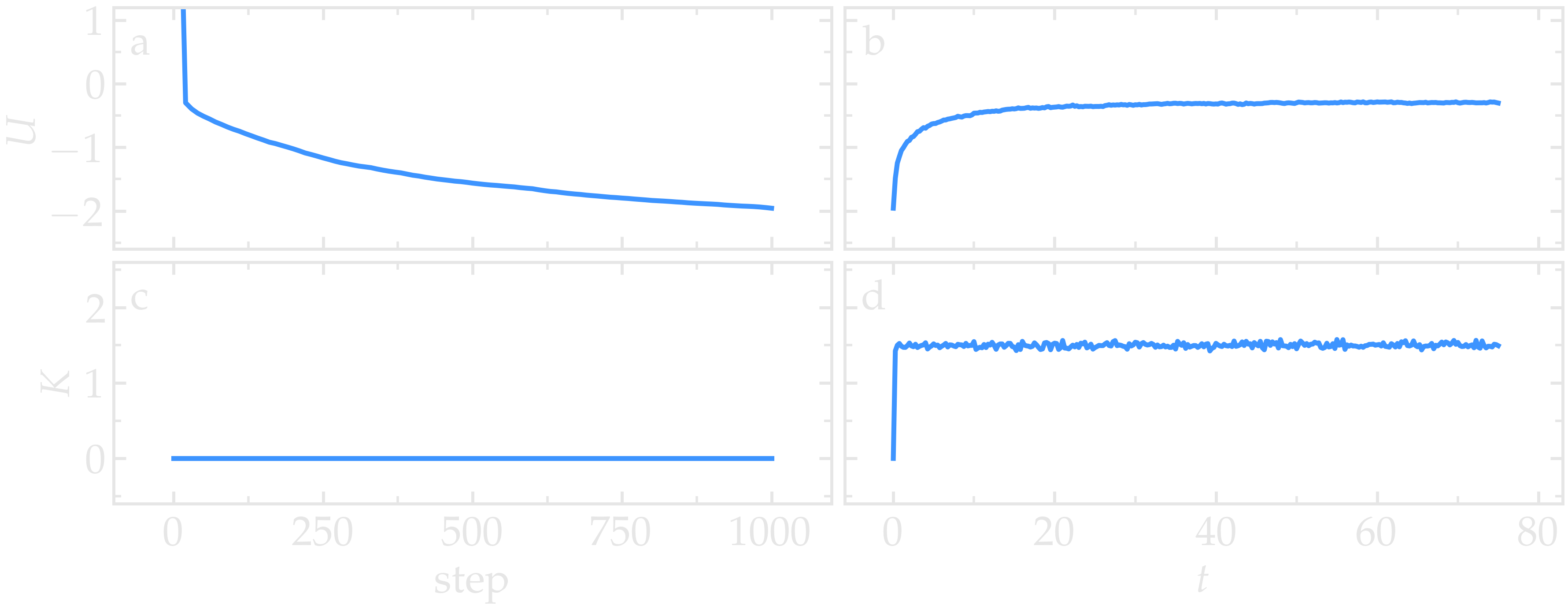
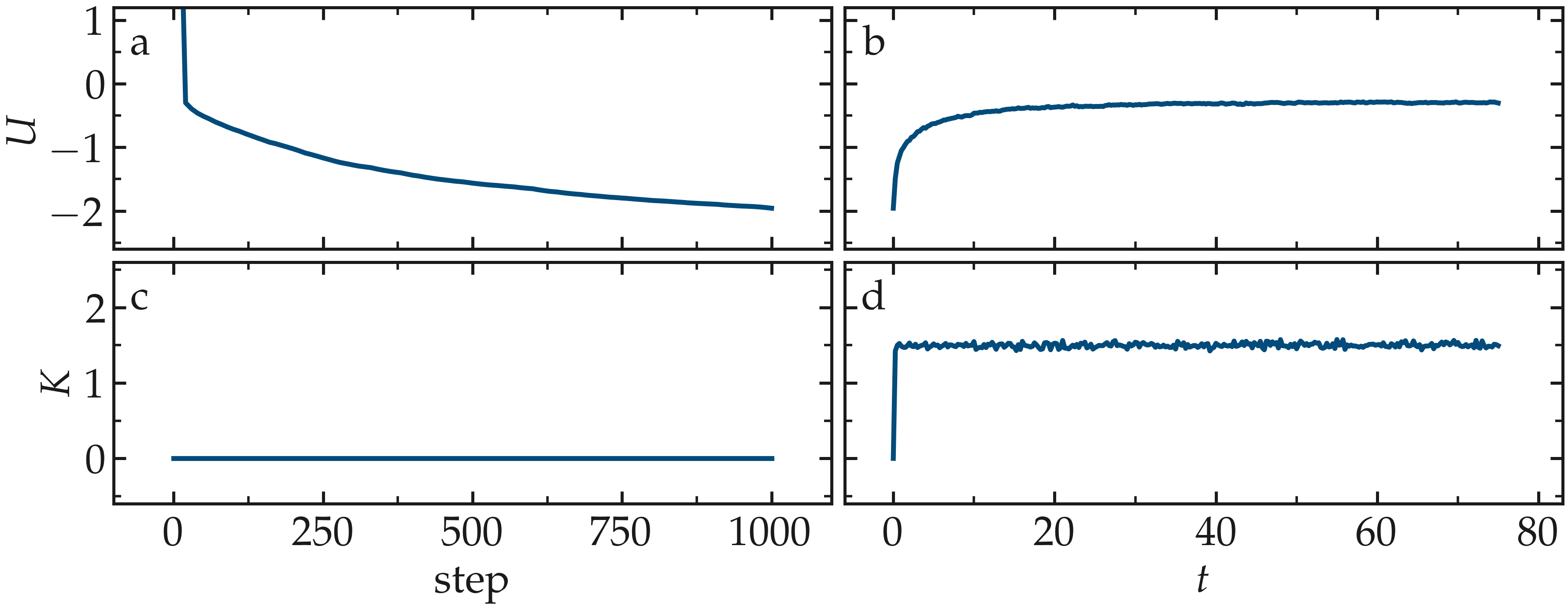
Figure: (a) Potential energy, \(U\), of the binary mixture as a function of the step during energy minimization. (b) Potential energy, \(U\), as a function of time, \(t\), during molecular dynamics in the NVT ensemble. (c) Kinetic energy, \(K\), during energy minimization. (d) Kinetic energy, \(K\), during molecular dynamics.

Trajectory visualization

So far, the simulation has been mostly monitored through the analysis of thermodynamic information. To better follow the evolution of the system and visualize the trajectories of the atoms, let us print the positions of the atoms in a file at a regular interval.

Add the following command to the Visualization section of PART B of the initial.lmp file:

dump mydmp all atom 100 dump.lammpstrj

Run the initial.lmp file using LAMMPS again. A file named dump.lammpstrj must appear alongside initial.lmp. The .lammpstrj file can be opened using VMD [12] or OVITO [13].

Use the dump image command to create snapshot images during the simulation. We have already explored the Image Viewer window. Open it again and adjust the visualization to your liking using the available buttons. Now you can copy the commands used to create this visualization to the clipboard by either using the Ctrl-D keyboard shortcut or selecting Copy dump image command from the File menu. This text can be pasted into the Visualization section of PART B of the initial.lmp file. This may look like the following:

dump viz all image 100 myimage-*.ppm type type size 800 800 zoom 1.452 shiny 0.7 fsaa yes &
    view 80 10 box yes 0.025 axes no 0.0 0.0 center s 0.483725 0.510373 0.510373
dump_modify viz pad 9 boxcolor royalblue backcolor white adiam 1 1.6 adiam 2 4.8

This command tells LAMMPS to generate NetPBM format images every 100 steps. The two type keywords are for color and diameter, respectively. Run the initial.lmp using LAMMPS again, and a new window named Slide Show will pop up. It will show each image created by the dump image as it is created. After the simulation is finished (or stopped), the slideshow viewer allows you to animate the trajectory by cycling through the images. The window also allows you to export the animation to a movie (provided the FFMpeg program is installed) and to bulk delete those image files.

The rendering of the system can be further adjusted using the many options of the dump image command. For instance, the value for the shiny keyword is used to adjust the shininess of the atoms, the box keyword adds or removes a representation of the box, and the view and zoom keywords adjust the camera (and so on).

Improving the script

Let us improve the input script and perform more advanced operations, such as specifying initial positions for the atoms and restarting the simulation from a previously saved configuration.

Control the initial atom positions

Open the improved.min.lmp, which was downloaded during the tutorial setup. This file contains the Part A of the initial.lmp file, but without any commands in the System definition section:

# 1) Initialization
units lj
dimension 3
atom_style atomic
boundary p p p
# 2) System definition
# 3) Settings
mass 1 1.0
mass 2 10.0
pair_style lj/cut 4.0
pair_coeff 1 1 1.0 1.0
pair_coeff 2 2 0.5 3.0
# 4) Visualization
thermo 10
thermo_style custom step etotal press
# 5) Run
minimize 1.0e-6 1.0e-6 1000 10000

We want to create the atoms of types 1 and 2 in two separate regions. To achieve this, we need to add two region commands and then reintroduce the create_atoms commands, this time using the new regions instead of the simulation box region to place the atoms:

# 2) System definition
region simbox block -20 20 -20 20 -20 20
create_box 2 simbox
# for creating atoms
region cyl_in cylinder z 0 0 10 INF INF side in
region cyl_out cylinder z 0 0 10 INF INF side out
create_atoms 1 random 1000 34134 cyl_out
create_atoms 2 random 150 12756 cyl_in

The side in and side out keywords are used to define regions representing the inside and outside of the cylinder of radius 10 length units. Then, append a sixth section titled Save system at the end of the file, ensuring that the write_data command is placed after the minimize command:

# 6) Save system
write_data improved.min.data

Note

A key improvement to the input is the addition of the write_data command. This command writes the state of the system to a text file called improved.min.data. This .data file will be used later to restart the simulation from the final state of the energy minimization step, eliminating the need to repeat the system creation and minimization.

Run the improved.min.lmp file using LAMMPS–GUI. At the end of the simulation, a file called improved.min.data is created.

You can view the contents of improved.min.data from LAMMPS–GUI, by right-clicking on the file name in the editor and selecting the entry View file improved.min.data.

The created .data file contains all the information necessary to restart the simulation, such as the number of atoms, the box size, the masses, and the pair coefficients. This .data file also contains the final positions of the atoms within the Atoms section. The first five columns of the Atoms section correspond (from left to right) to the atom indexes (from 1 to the total number of atoms, 1150), the atom types (1 or 2 here), and the positions of the atoms \(x\), \(y\), \(z\). The last three columns are image flags that keep track of which atoms crossed the periodic boundary. The exact format of each line in the Atoms section depends on the choice of atom_style, which determines which per-atom data is set and stored internally in LAMMPS.

Note

Instead of the write_data command, you can also use the write_restart command to save the state of the simulation to a binary restart file. Binary restart files are more compact, faster to write, and contain more information, making them often more convenient to use. For example, the choice of atom_style or pair_style is recorded, so those commands do not need to be issued before reading the restart. Note however that restart files are not expected to be portable across LAMMPS versions or platforms. Therefore, in these tutorials, and with the exception of Tutorial 3, Polymer in water, we primarily use write_data to provide you with a reference copy of the data file that works regardless of your LAMMPS version and platform.

Restarting from a saved configuration

To continue a simulation from the saved configuration, open the improved.md.lmp file, which was downloaded during the tutorial setup. This file contains the Initialization part from initial.lmp and improved.min.lmp:

# 1) Initialization
units lj
dimension 3
atom_style atomic
boundary p p p
# 2) System definition
# 3) Settings
# 4) Visualization
# 5) Run

Since we read most of the information from the data file, we don’t need to repeat all the commands from the System definition and Settings categories. The exception is the pair_style command, which now must come before the simulation box is defined, meaning before the read_data command. Add the following lines to improved.md.lmp:

# 2) System definition
pair_style lj/cut 4.0
read_data improved.min.data

By visualizing the system, you may have noticed that some atoms left their original region during minimization. To start the simulation from a clean slate, with only atoms of type 2 inside the cylinder and atoms of type 1 outside the cylinder, let us delete the misplaced atoms by adding the following commands to improved.md.lmp:

region cyl_in cylinder z 0 0 10 INF INF side in
region cyl_out cylinder z 0 0 10 INF INF side out
group grp_t1 type 1
group grp_t2 type 2
group grp_in region cyl_in
group grp_out region cyl_out
group grp_t1_in intersect grp_t1 grp_in
group grp_t2_out intersect grp_t2 grp_out
delete_atoms group grp_t1_in
delete_atoms group grp_t2_out

The first two region commands recreate the previously defined regions, which is necessary since regions are not saved by the write_data command. The first two group commands create groups containing all the atoms of type 1 and all the atoms of type 2, respectively. The next two group commands create atom groups based on their positions at the beginning of the simulation, i.e., when the commands are being read by LAMMPS. The last two group commands create atom groups based on the intersection between the previously defined groups. Finally, the two delete_atoms commands delete the atoms of type 1 located inside the cylinder and the atoms of type 2 located outside the cylinder, respectively.

Since LAMMPS has a limited number of custom groups (30), it is good practice to delete groups that are no longer needed. This can be done by adding the following four commands to improved.md.lmp:

# delete no longer needed groups
group grp_in delete
group grp_out delete
group grp_t1_in delete
group grp_t2_out delete

Let us monitor the number of atoms of each type inside the cylinder as a function of time by creating the following equal-style variables:

variable n1_in equal count(grp_t1,cyl_in)
variable n2_in equal count(grp_t2,cyl_in)

The equal-style variables are expressions evaluated during the run and return a number. Here, they are defined to count the number of atoms of a specific group within the cyl_in region.

In addition to counting the atoms in each region, we will also extract the coordination number of type 2 atoms around type 1 atoms. The coordination number measures the number of type 2 atoms near type 1 atoms, defined by a cutoff distance. Taking the average provides a good indicator of the degree of mixing in a binary mixture. This is done using two compute commands: the first counts the coordinated atoms, and the second calculates the average over all type 1 atoms. Add the following lines to improved.md.lmp:

compute coor12 grp_t1 coord/atom cutoff 2 group grp_t2
compute sumcoor12 grp_t1 reduce ave c_coor12

The compute reduce ave command is used to average the per-atom coordination number calculated by the coord/atom compute command. Compute commands are not automatically invoked; they require a consumer command that references the compute. In this case, the first compute is referenced by the second, and we reference the second in a thermo_style custom command (see below).

Note

There is no need for a Settings section, as the settings are taken from the .data file.

Finally, let us complete the script by adding the following lines to improved.md.lmp:

# 4) Visualization
thermo 1000
thermo_style custom step temp pe ke etotal press v_n1_in v_n2_in c_sumcoor12
dump viz all image 1000 myimage-*.ppm type type shiny 0.1 box no 0.01 view 0 0 zoom 1.8 fsaa yes size 800 800
dump_modify viz adiam 1 1 adiam 2 3 acolor 1 turquoise acolor 2 royalblue backcolor white

The two variables n1_in, n2_in, along with the compute sumcoor12, were added to the list of information printed during the simulation. Additionally, images of the system will be created with slightly less saturated colors than the default ones.

Finally, add the following lines to improved.md.lmp:

# 5) Run
velocity all create 1.0 49284 mom yes dist gaussian
fix mynve all nve
fix mylgv all langevin 1.0 1.0 0.1 10917 zero yes
timestep 0.005
run 300000

Here, there are a few more differences from the previous simulation. First, the velocity create command assigns an initial velocity to each atom. The initial velocity is chosen so that the average initial temperature is equal to 1.0 temperature units. The additional keywords ensure that no linear momentum (mom yes) is given to the system and that the generated velocities are distributed according to a Gaussian distribution. Another improvement is the zero yes keyword in the Langevin thermostat, which ensures that the total random force applied to the atoms is equal to zero. These steps are important to prevent the system from starting to drift or move as a whole.

Note

A bulk system with periodic boundary conditions is expected to remain in place. Accordingly, when computing the temperature from the kinetic energy, we use \(3N-3`\) degrees of freedom since there is no global translation. In a drifting system, some of the kinetic energy is due to the drift, which means the system itself cools down. In extreme cases, the system can freeze while its center of mass drifts very quickly. This phenomenon is sometimes referred to as the flying ice cube syndrome [19].

Run improved.md.lmp and observe the mixing of the two populations over time.

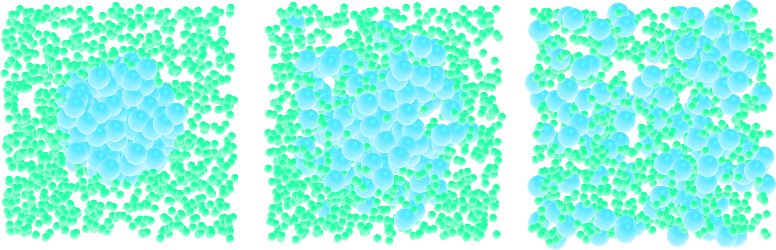
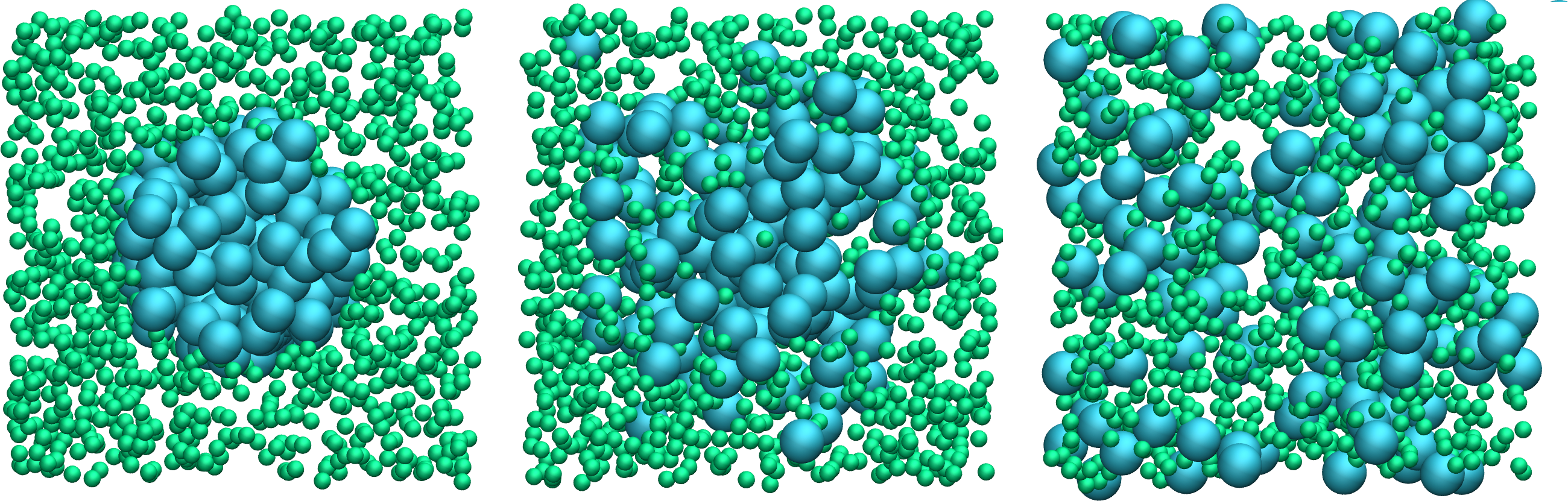
Figure: Evolution of the system during mixing. The three snapshots show respectively the system at \(t = 0\) (left panel), \(t = 75\) (middle panel), and \(t = 1500\) (right panel). The atoms of type 1 are represented as small green spheres and the atoms of type 2 as large cyan spheres.

From the variables n1_in and n2_in, you can track the number of atoms in each region as a function of time (figure below, panel a). To view their evolution, select the entries v_n1_in or v_n2_in in the Data drop-down menu in the Charts window of LAMMPS–GUI. In addition, as the mixing progresses, the average coordination number between atoms of types 1 and 2 increases from about 0.01 to 0.04 (figure below, panel b). This indicates that, over time, more and more particles of type 1 come into contact with particles of type 2, as expected during mixing. This can be observed using the entry c_sumcoor12 in the Charts drop-down menu.

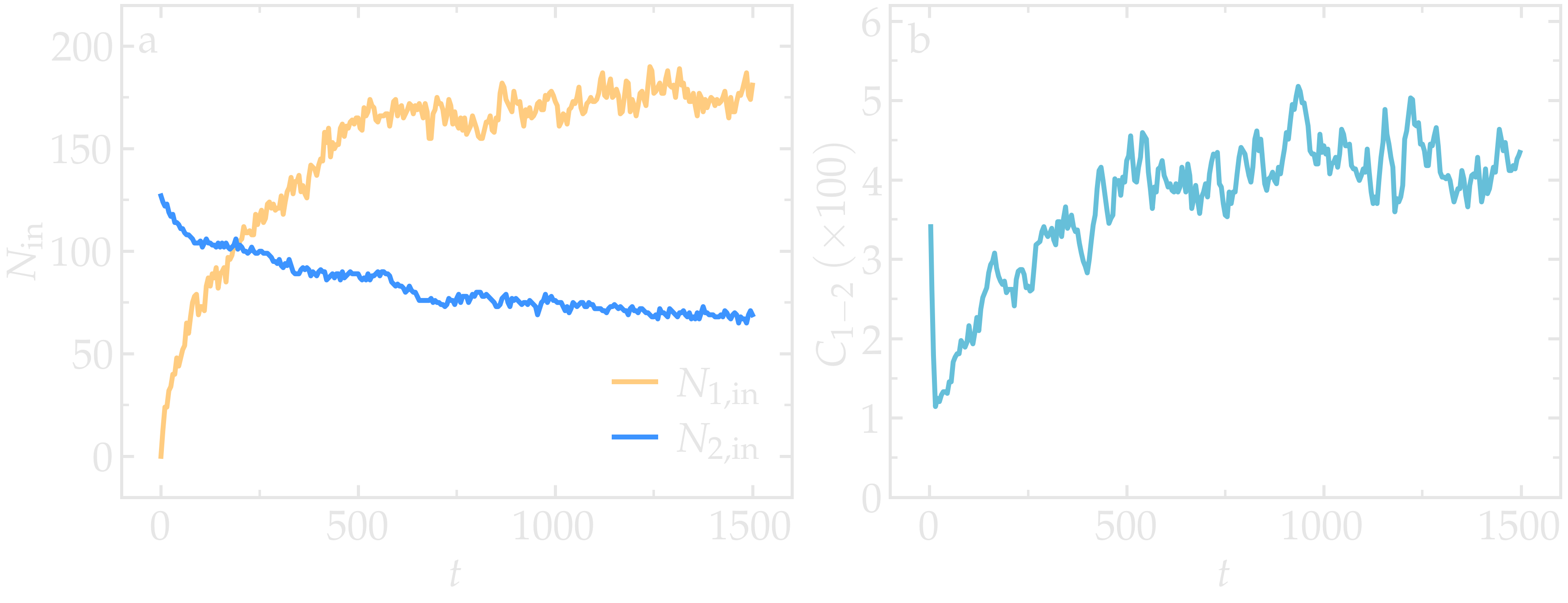
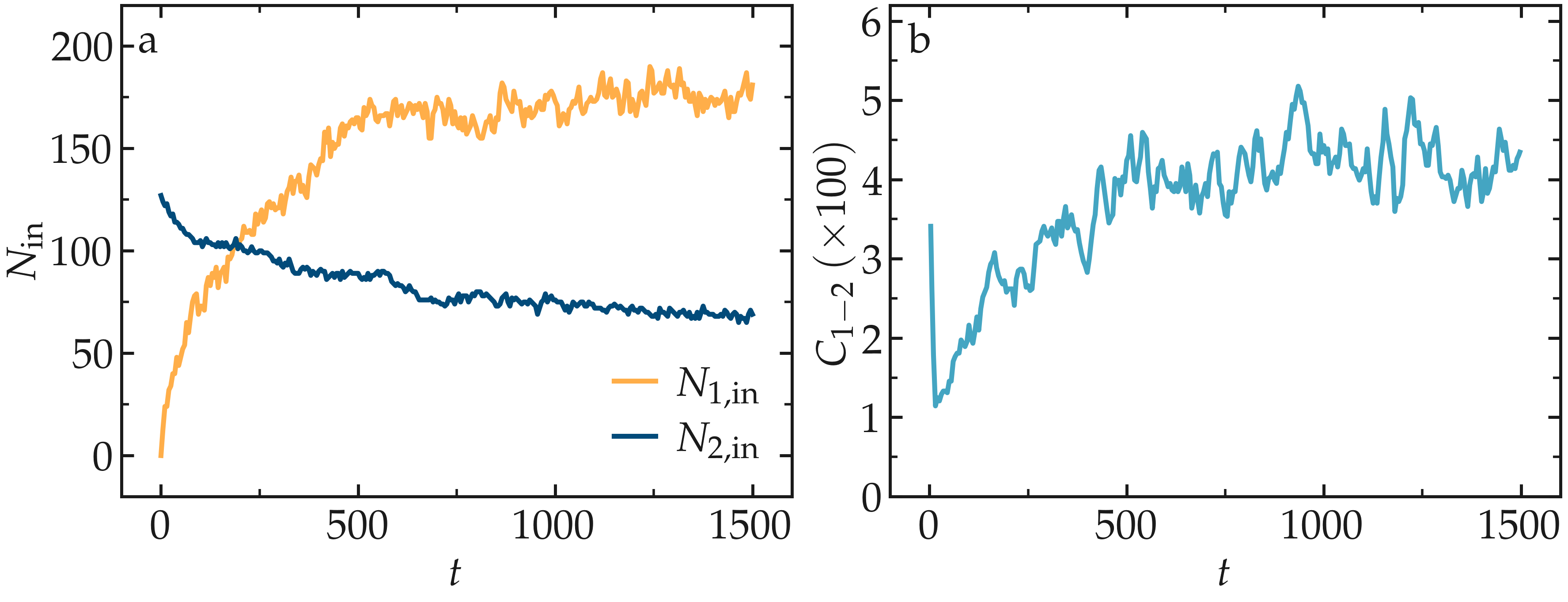
Figure: a) Evolution of the numbers \(N_\text{1, in}$\) and \(N_\text{2, in}\) of atoms of types 1 and 2, respectively, within the cyl_in region as functions of time \(t\). b) Evolution of the coordination number \(C_{1-2}\) (compute sumcoor12) between atoms of types 1 and 2.

Cite

You can access the input scripts and data files that are used in these tutorials from a dedicated Github repository. This repository also contains the full solutions to the exercises.

Going further with exercises

Experiments

Here are some suggestions for further experiments with this system that may lead to additional insights into how different systems are configured and how various features function:

• Use a Nosé-Hoover thermostat (fix nvt) instead of a Langevin thermostat (fix nve + fix langevin).

• Omit the energy minimization step before starting the MD simulation using either the Nosé-Hoover or the Langevin thermostat.

• Apply a thermostat to only one type of atoms and observe the temperature for each type separately.

• Append an NVE run (i.e., without any thermostat) and observe the energy levels.

If you are using LAMMPS-GUI

An useful experiment is coloring the atoms in the Slide Show according to an observable, such as their respective coordination numbers. To do this, replace the dump and dump_modify commands with the following lines:

variable coor12 atom (type==1)*(c_coor12)+(type==2)*-1
dump viz all image 1000 myimage-*.ppm v_coor12 type &
shiny 0.1 box no 0.01 view 0 0 zoom 1.8 fsaa yes size 800 800
dump_modify viz adiam 1 1 adiam 2 3 backcolor white &
amap -1 2 ca 0.0 4 min royalblue 0 turquoise 1 yellow max red

Run LAMMPS again. Atoms of type 1 are now colored based on the value of c_coor12, which is mapped continuously from turquoise to yellow and red for atoms with the highest coordination. In the definition of the variable v_coor12, atoms of type 2 are all assigned a value of -1, and will therefore always be colored their default blue.

Solve Lost atoms error

For this exercise, the following input script is provided:

units lj
dimension 3
atom_style atomic
pair_style lj/cut 2.5
boundary p p p

region simulation_box block -20 20 -20 20 -20 20
create_box 1 simulation_box
create_atoms 1 random 1000 341841 simulation_box

mass 1 1
pair_coeff 1 1 1.0 1.0

dump mydmp all atom 100 dump.lammpstrj
thermo 100
thermo_style custom step temp pe ke etotal press

fix mynve all nve
fix mylgv all langevin 1.0 1.0 0.1 1530917
timestep 0.005

run 10000

As it is, this input returns one of the most common error that you will encounter using LAMMPS:

ERROR: Lost atoms: original 1000 current 984

The goal of this exercise is to fix the Lost atoms error without using any other command than the ones already present. You can only play with the values of the parameters and/or replicate every command as many times as needed.

Note

This script is failing because particles are created randomly in space, some of them are likely overlapping, and no energy minimization is performed prior to start the molecular dynamics simulation.

Create a demixed dense phase

Starting from one of the input created in this tutorial, fine-tune the parameters such as particle numbers and interaction to create a simulation with the following properties:

• the density in particles must be high,

• both particles of type 1 and 2 must have the same size,

• particles of type 1 and 2 must demix.

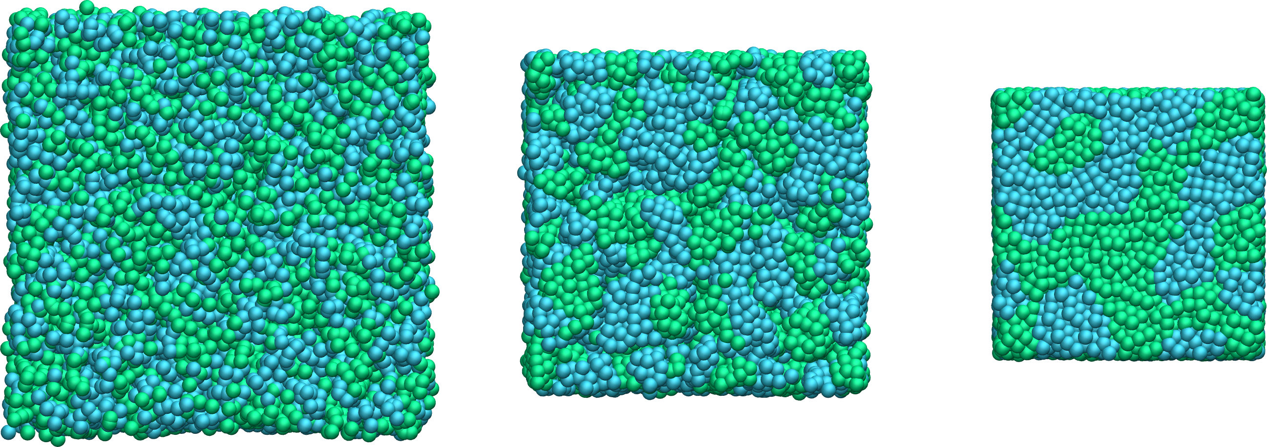
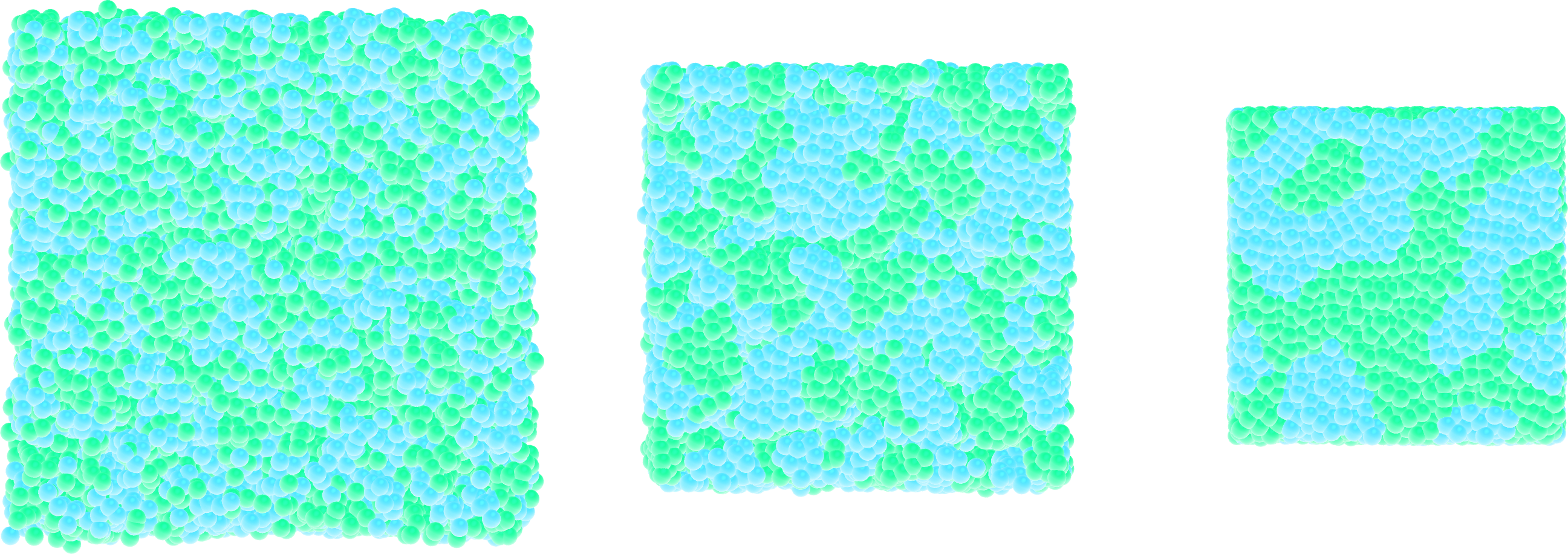
Figure: Snapshots taken at different times showing the particles of type 1 and type 2 progressively demixing and forming large demixed areas.

Hint

An easy way to create a dense phase is to allow the box dimensions to relax until the vacuum disappears. You can do that by replacing the fix nve with fix nph.

From atoms to molecules

Add a bond between particles of type 2 to create dumbbell molecules instead of single particles.

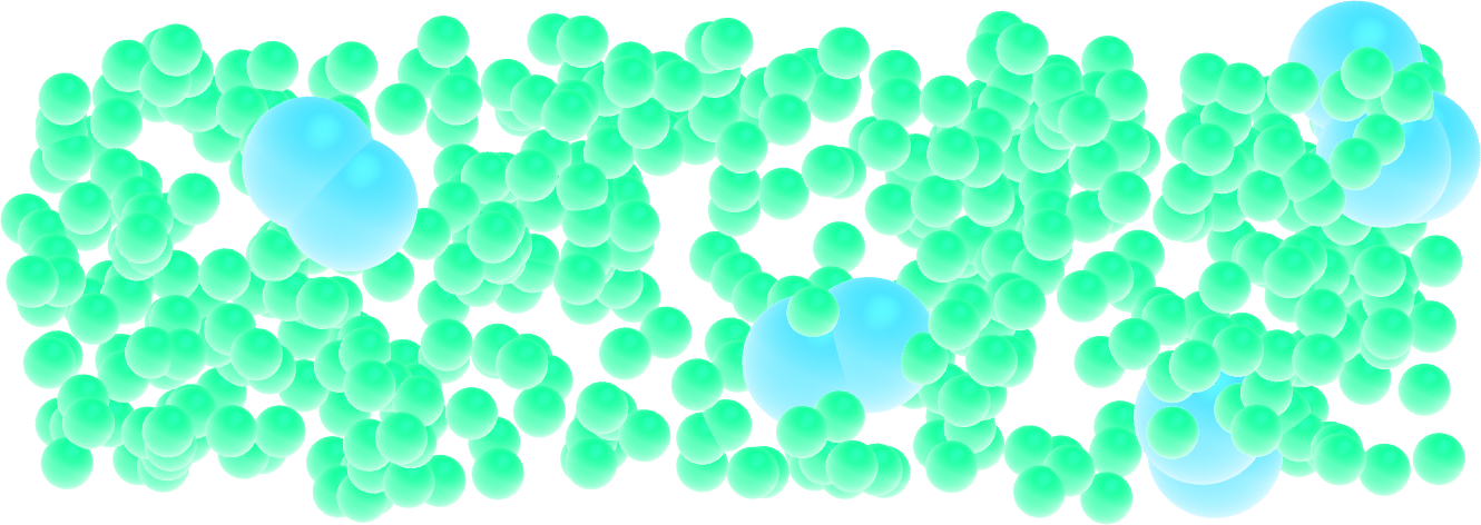
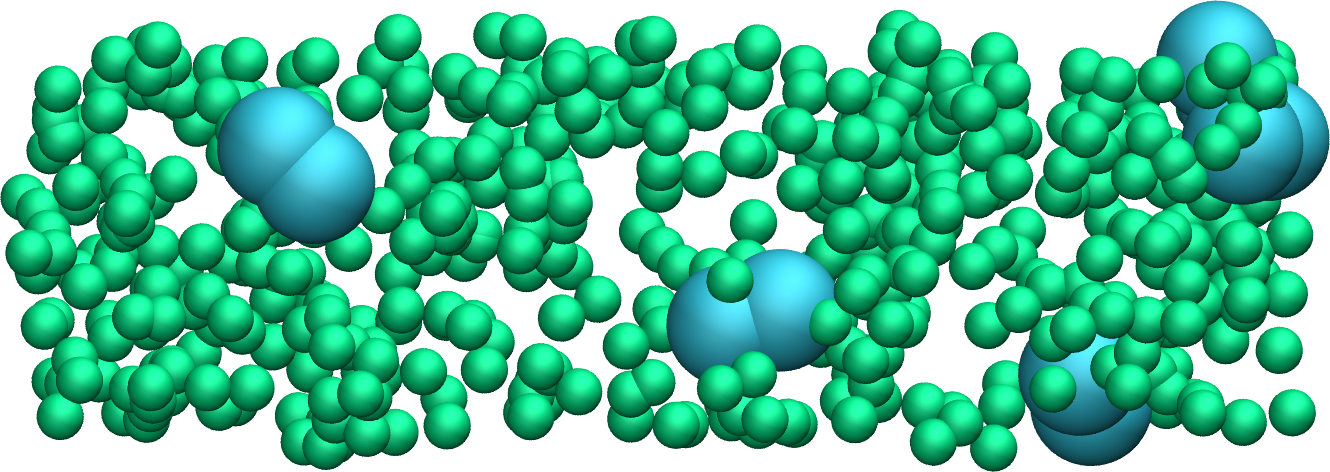
Figure: Dumbbell molecules made of 2 large spheres mixed with smaller particles (small spheres). See the corresponding video.

Similarly to the dumbbell molecules, create a small polymer, i.e. a long chain of particles linked by bonds and angles.

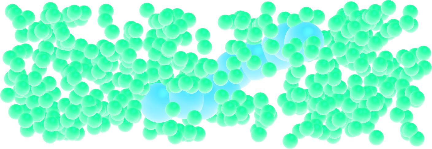
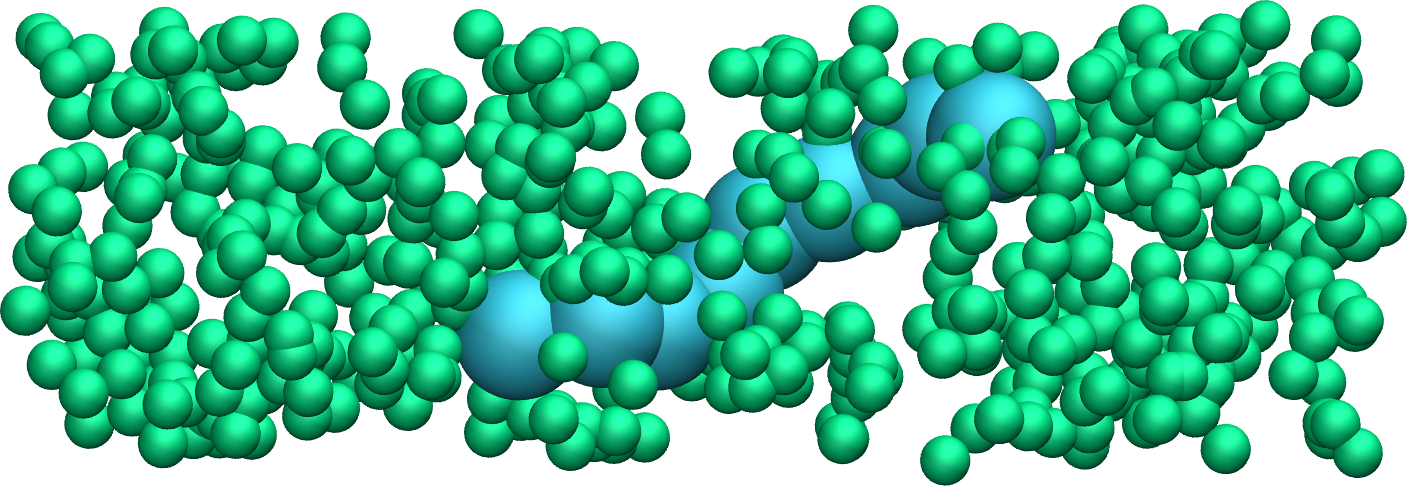
Figure: A single small polymer molecule made of 9 large spheres mixed with smaller particles. See the corresponding video.

Hints

Use a molecule template to easily insert as many atoms connected by bonds (i.e. molecules) as you want. A molecule template typically begins as follows:

2 atoms
1 bonds

Coords

1 0.5 0 0
2 -0.5 0 0

(...)

A bond section also needs to be added, see this page for details on the formatting of a molecule template.