Polymer in water

Solvating and stretching a small polymer molecule

The goal of this tutorial is to use LAMMPS to solvate a small hydrophilic polymer (PEG - polyethylene glycol) in a reservoir of water.

Once the water reservoir is properly equilibrated at the desired temperature and pressure, the polymer molecule is added and a constant stretching force is applied to both ends of the polymer. The evolution of the polymer length is measured as a function of time. The GROMOS 54A7 force field [23] is used for the PEG, the SPC/Fw model [24] is used for the water, and the long-range Coulomb interactions are solved using the PPPM solver [25].

This tutorial was inspired by a publication by Liese and coworkers, in which molecular dynamics simulations are compared with force spectroscopy experiments, see Ref. [26].

If you are completely new to LAMMPS, we recommend that you follow this tutorial on a simple Lennard-Jones fluid first.

Cite

If you find these tutorials useful, you can cite A Set of Tutorials for the LAMMPS Simulation Package by Simon Gravelle, Jacob R. Gissinger, and Axel Kohlmeyer (2025) [14]. You can access the full paper on arXiv.

This tutorial is compatible with the 29Aug2024 (update 2) LAMMPS version.

Preparing the water reservoir

In this tutorial, the water reservoir is first prepared in the absence of the polymer. A rectangular box of water is created and equilibrated at ambient temperature and pressure. The SPC/Fw water model is used [24], which is a flexible variant of the rigid SPC (simple point charge) model [27]. Create a file named water.lmp, and copy the following lines into it:

units real
atom_style full
bond_style harmonic
angle_style harmonic
dihedral_style harmonic
pair_style lj/cut/coul/long 10
kspace_style ewald 1e-5
special_bonds lj 0.0 0.0 0.5 coul 0.0 0.0 1.0 angle yes

Optional: follow this tutorial using LAMMPS-GUI

To set up this tutorial, select Start Tutorial 3 from the Tutorials menu of LAMMPS–GUI and follow the instructions. The editor should display the content corresponding to water.lmp.

With the unit style real, masses are in g/mol, distances in Å, time in fs, and energies in kcal/mol. With the atom_style full, each atom is a dot with a mass and a charge that can be linked by bonds, angles, dihedrals, and/or impropers. The bond_style, angle_style, and dihedral_style commands define the potentials for the bonds, angles, and dihedrals used in the simulation, here harmonic. With the pair_style named lj/cut/coul/long, atoms interact through both a Lennard-Jones (LJ) potential and Coulomb interactions. The value of \(10\,\text{Å}\) is the cutoff, and the ewald command defines the long-range solver for the Coulomb interactions [28]. Finally, the special_bonds command, which was already seen in Pulling on a carbon nanotube, sets the LJ and Coulomb weighting factors for the interaction between neighboring atoms.

Let us create a 3D simulation box of dimensions \(6 \times 3 \times 3 \; \text{nm}^3\), and make space for 8 atom types (2 for the water, 6 for the polymer), 7 bond types (1 for the water, 6 for the polymer), 8 angle types (1 for the water, 7 for the polymer), and 4 dihedral types (only for the polymer). Copy the following lines into water.lmp:

region box block -30 30 -15 15 -15 15
create_box 8 box bond/types 7 angle/types 8 dihedral/types 4 extra/bond/per/atom 3 &
    extra/angle/per/atom 6 extra/dihedral/per/atom 10 extra/special/per/atom 14

The extra/x/per/atom commands reserve memory for adding bond topology data later. We use the file parameters.inc to set all the parameters (masses, interaction energies, bond equilibrium distances, etc). Thus add to water.lmp the line:

include parameters.inc

Note

This tutorial uses type labels [3] to map each numeric atom type to a string (see the parameters.inc file): labelmap atom 1 OE 2 C 3 HC 4 H 5 CPos 6 OAlc 7 OW 8 HW Therefore, the oxygen and hydrogen atoms of water (respectively types 7 and 8) can be referred to as OW and HW, respectively. Similar maps are used for the bond types, angle types, and dihedral types.

Let us create water molecules. To do so, let us import a molecule template called water.mol and then randomly create 700 molecules. Add the following lines into water.lmp:

molecule h2omol water.mol
create_atoms 0 random 700 87910 NULL mol h2omol 454756 overlap 1.0 maxtry 50

The overlap 1.0 option of the create_atoms command ensures that no atoms are placed exactly in the same position, as this would cause the simulation to crash. The maxtry 50 asks LAMMPS to try at most 50 times to insert the molecules, which is useful in case some insertion attempts are rejected due to overlap. In some cases, depending on the system and the values of overlap and maxtry, LAMMPS may not create the desired number of molecules. Always check the number of created atoms in the log file (or in the Output window), where you should see:

Created 2100 atoms

When LAMMPS fails to create the desired number of molecules, a WARNING appears. The molecule template called water.mol must be downloaded and saved next to water.lmp. This template contains the necessary structural information of a water molecule, such as the number of atoms, or the IDs of the atoms that are connected by bonds and angles.

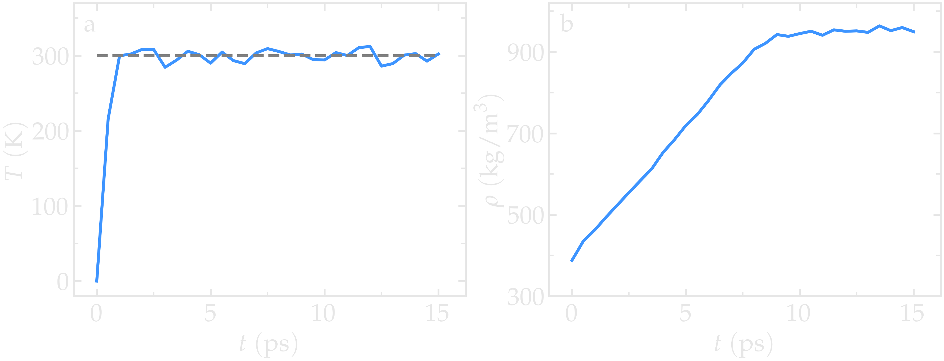
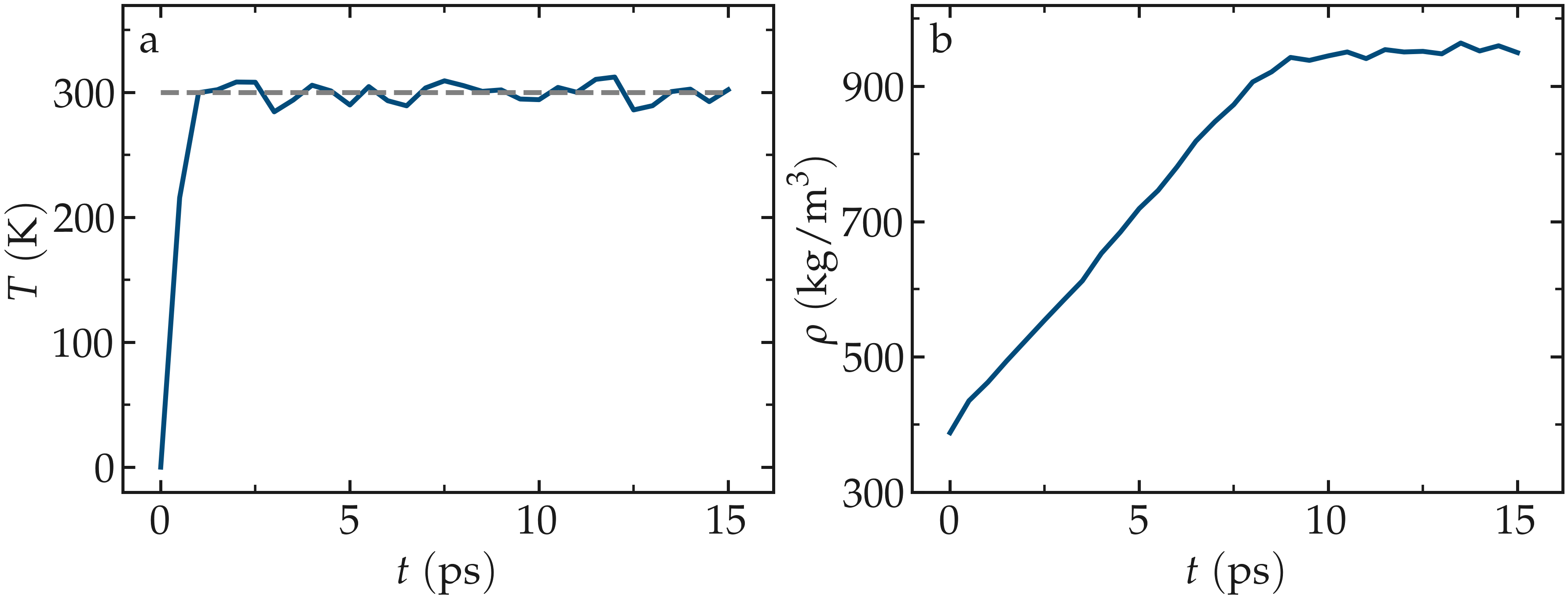
Figure: a) Temperature, \(T\), of the water reservoir as a function of the time, \(t\). The horizontal dashed line is the target temperature of \(300 \text{K}\). b) Evolution of the system density, \(\rho\), with \(t\)

Then, let us organize the atoms of types OW and HW of the water molecules in a group named H2O and perform a small energy minimization. The energy minimization is mandatory here because of the small overlap value of 1 Å chosen in the create_atoms command. Add the following lines into water.lmp:

group H2O type OW HW
minimize 1.0e-4 1.0e-6 100 1000
reset_timestep 0

Resetting the step of the simulation to 0 using the reset_timestep command is optional. It is used here because the number of iterations performed by the minimize command is usually not a round number, since the minimization stops when one of four criteria is reached. We will use fix npt to control the temperature and pressure of the molecules with a Nosé-Hoover thermostat and barostat, respectively [21, 22, 29]. Add the following line into water.lmp:

fix mynpt all npt temp 300 300 100 iso 1 1 1000

The fix npt allows us to impose both a temperature of \(300\,\text{K}\) (with a damping constant of \(100\,\text{fs}\)), and a pressure of 1 atmosphere (with a damping constant of \(1000\,\text{fs}\)). With the iso keyword, the three dimensions of the box will be re-scaled simultaneously.

Let us output the system into images by adding the following commands to water.lmp:

dump viz all image 250 myimage-*.ppm type type &
shiny 0.1 box no 0.01 view 0 90 zoom 3 size 1000 600
dump_modify viz backcolor white &
acolor OW red acolor HW white &
adiam OW 3 adiam HW 1.5

Let us also extract the volume and density every 500 steps:

variable myvol equal vol
variable myoxy equal count(H2O)/3
variable NA equal 6.022e23
variable Atom equal 1e-10
variable M equal 0.018
variable rho equal ${myoxy}*${M}/(v_myvol*${NA}*${Atom}^3)
thermo 500
thermo_style custom step temp etotal v_myvol v_rho

Here, several variables are defined and used for converting the units of the density in kg/mol: The variable myoxy represents the number of atoms divided by 3, which corresponds to the number of molecules, \(N_\text{H2O}\), and the variable myrho is the density in kg/mol:

\[\rho = \dfrac{N_\text{H2O}}{V N_\text{A}},\]

where \(V\) is the volume in \(\text{m}^3\), \(N_\text{A}\) the Avogadro number, and \(M = 0.018\),kg/mol the molar mass of water.

Finally, let us set the timestep to 1.0 fs, and run the simulation for 15 ps by adding the following lines into water.lmp:

timestep 1.0
run 15000

write_restart water.restart

The final state is saved in a binary file named water.restart. Run the input using LAMMPS. The system reaches its equilibrium temperature after just a few picoseconds, and its equilibrium density after approximately 10 picoseconds.

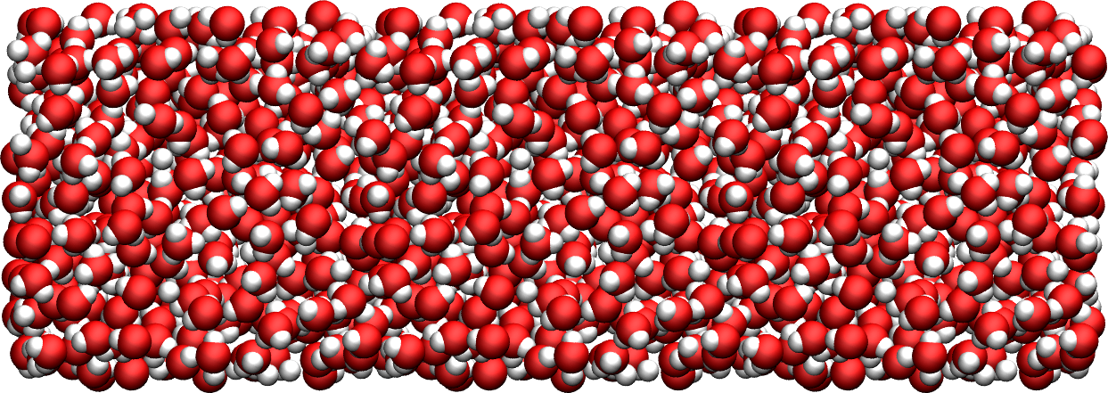
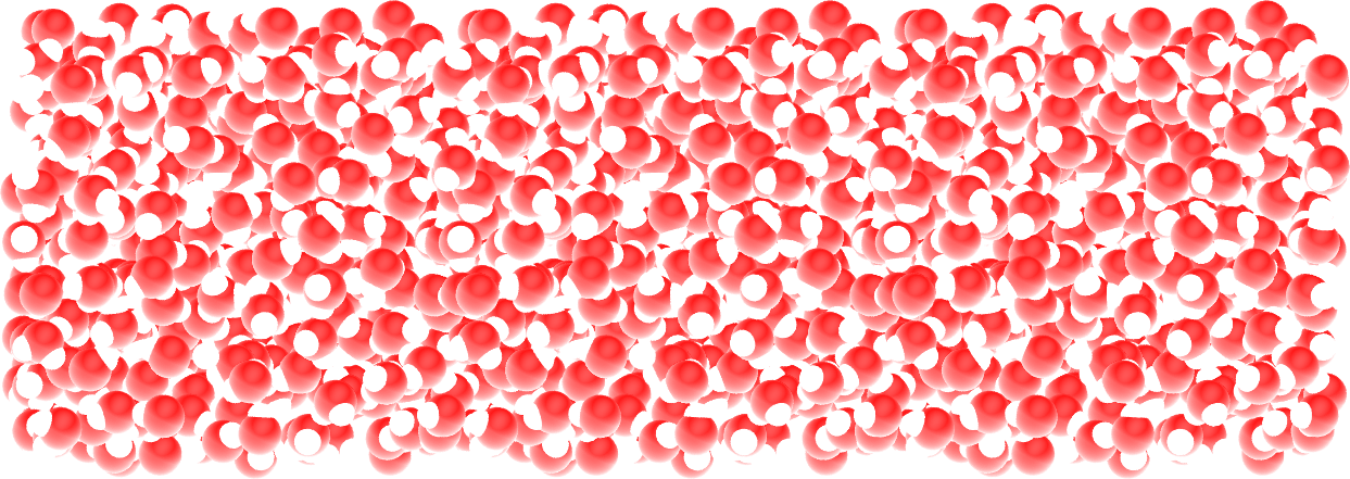
Figure: The water reservoir after equilibration. Oxygen atoms are in red, and hydrogen atoms are in white.

Note

The binary file created by the write_restart command contains the complete state of the simulation, including atomic positions, velocities, and box dimensions (similar to write_data), but also the groups, the compute, or the atom_style. Use the Inspect Restart option of the LAMMPS–GUI to vizualize the content saved in water.restart.

Solvating the PEG in water

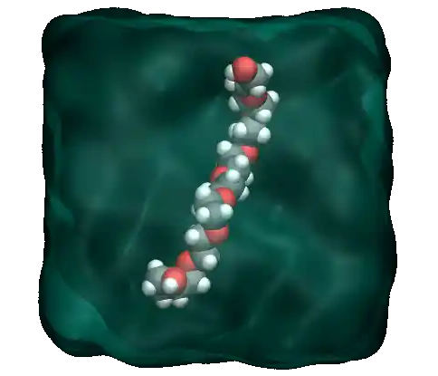
Now that the water reservoir is equilibrated, we can safely add the PEG polymer to the water. The PEG molecule topology was downloaded from the ATB repository [30, 31]. It has a formula \(\text{C}_{16}\text{H}_{34}\text{O}_{9}\), and the parameters are taken from the GROMOS 54A7 force field [23].

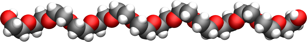
Figure: The PEG molecule with carbon atoms in gray, oxygen atoms in red, and hydrogen atoms in white.

Open the file named merge.lmp that was downloaded alongside water.lmp during the tutorial setup. It only contain one line:

read_restart water.restart

Most of the commands that were initially present in water.lmp, such as the units of the atom_style commands do not need to be repeated, as they were saved within the .restart file. There is also no need to re-include the parameters from the .inc file. The kspace_style command, however, is not saved by the write_restart command and must be repeated. Since Ewald summation is not the most efficient choice for such dense system, let us use PPPM (for particle-particle particle-mesh) for the rest of the tutorial. Add the following command to merge.lmp:

kspace_style pppm 1e-5

Using the molecule template for the polymer called peg.mol, let us create a single molecule in the middle of the box by adding the following commands to merge.lmp:

molecule pegmol peg.mol
create_atoms 0 single 0 0 0 mol pegmol 454756

Let us create a group for the atoms of the PEG (the previously created group H2O was saved by the restart and can be omitted):

group PEG type C CPos H HC OAlc OE

Water molecules that are overlapping with the PEG must be deleted to avoid future crashing. Add the following line into merge.lmp:

delete_atoms overlap 2.0 H2O PEG mol yes

Here the value of 2.0 Å for the overlap cutoff was fixed arbitrarily and can be chosen through trial and error. If the cutoff is too small, the simulation will crash because atoms that are too close to each other undergo forces that can be extremely large. If the cutoff is too large, too many water molecules will unnecessarily be deleted.

Let us use the fix npt to control the temperature, as well as the pressure by allowing the box size to be rescaled along the \(x\)-axis:

fix mynpt all npt temp 300 300 100 x 1 1 1000

Let us also use the recenter command to always keep the PEG at the position \((0, 0, 0)\):

fix myrct PEG recenter 0 0 0 shift all

Note that the recenter command has no impact on the dynamics, it simply repositions the frame of reference so that any drift of the system is ignored, which can be convenient for visualizing and analyzing the system.

Let us create images of the systems:

dump viz all image 250 myimage-*.ppm type type size 1100 600 box no 0.1 shiny 0.1 view 0 90 zoom 3.3 fsaa yes bond atom 0.8
dump_modify viz backcolor white acolor OW red adiam OW 0.2 acolor OE darkred adiam OE 2.6 acolor HC white adiam HC 1.4 &
    acolor H white adiam H 1.4 acolor CPos gray adiam CPos 2.8 acolor HW white adiam HW 0.2 acolor C gray  adiam C 2.8 &
    acolor OAlc darkred adiam OAlc 2.6
thermo 500

Finally, to perform a short equilibration and save the final state to a .restart file, add the following lines to the input:

timestep 1.0
run 10000

write_restart merge.restart

Run the simulation using LAMMPS. From the outputs, you can make sure that the temperature remains close to the target value of \(300~\text{K}\) throughout the entire simulation, and that the volume and total energy are almost constant, indicating that the system was in a reasonable configuration from the start.

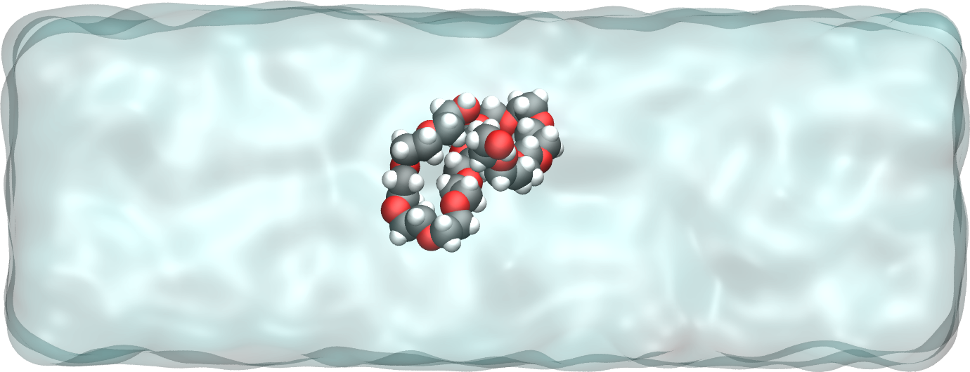
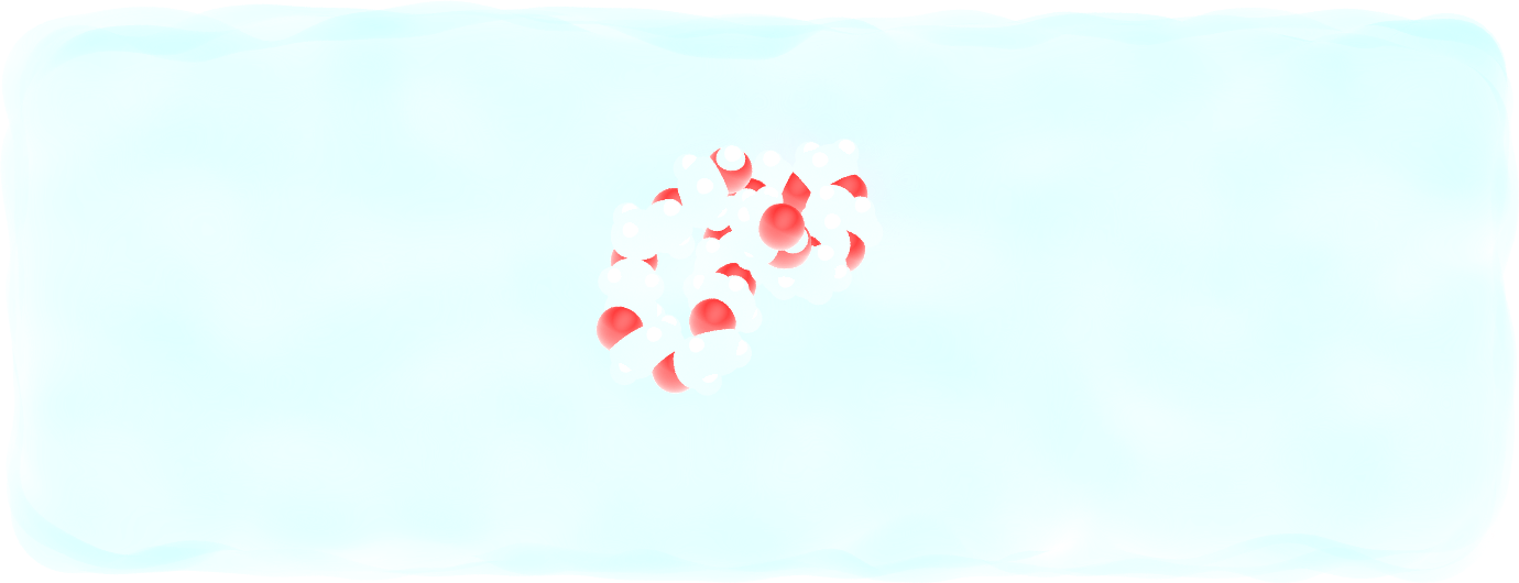
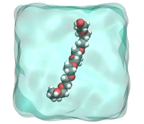
Figure : The PEG molecule solvated in water. Water is represented as a transparent field for clarity.

Stretching the PEG molecule

Here, a constant force is applied to both ends of the PEG molecule until it stretches. Open the file named pull.lmp, which only contains two lines:

kspace_style pppm 1e-5
read_restart merge.restart

Next, we’ll create new atom groups, each containing a single oxygen atom. The atoms of type OAlc correspond to the hydroxyl (alcohol) group oxygen atoms located at the ends of the PEG molecule, which we will use to apply the force. Add the following lines to pull.lmp:

group ends type OAlc
variable xcm equal xcm(ends,x)
variable oxies atom type==label2type(atom,OAlc)
variable end1 atom v_oxies*(x>v_xcm)
variable end2 atom v_oxies*(x<v_xcm)
group topull1 variable end1
group topull2 variable end2

These lines identify the oxygen atoms (type OAlc) at the ends of the PEG molecule and calculates their center of mass along the \(x\)-axis. It then divides these atoms into two groups, end1 (i.e., the OAlc atom to the right of the center) and end2 (i.e., the OAlc atom to the right of the center), for applying force during the stretching process.

Add the following dump command to create images of the system:

dump viz all image 250 myimage-*.ppm type type shiny 0.1 box no 0.01 &
    view 0 90 zoom 3.3 fsaa yes bond atom 0.8 size 1100 600
dump_modify viz backcolor white acolor OW red acolor HW white acolor OE darkred acolor OAlc darkred acolor C gray acolor CPos gray &
    acolor H white acolor HC white adiam OW 0.2 adiam HW 0.2 adiam C 2.8 adiam CPos 2.8 adiam OAlc 2.6 adiam H 1.4 adiam HC 1.4 adiam OE 2.6

Let us use a single Nosé-Hoover thermostat applied to all the atoms, and let us keep the PEG in the center of the box, by adding the following lines to pull.lmp:

timestep 1.0
fix mynvt all nvt temp 300 300 100
fix myrct PEG recenter 0 0 0 shift all

To investigate the stretching of the PEG molecule, let us compute its radius of gyration [32] and the angles of its dihedral constraints using the following commands:

compute rgyr PEG gyration
compute prop PEG property/local dtype
compute dphi PEG dihedral/local phi

The radius of gyration can be directly printed with the thermo_style command:

thermo_style custom step temp etotal c_rgyr
thermo 250
dump mydmp all local 100 pull.dat index c_dphi c_prop

By contrast with the radius of gyration (compute rgyr), the dihedral angle \(\phi\) (compute dphi) is returned as a vector by the compute dihedral/local command and must be written to a file using the dump local command.

Finally, let us simulate 15 picoseconds without any external force:

run 15000

This initial run will serve as a benchmark to quantify the changes caused by the applied force in later steps. Next, let us apply a force to the two selected oxygen atoms using two addforce commands, and then run the simulation for an extra 15 ps:

fix myaf1 topull1 addforce 10 0 0
fix myaf2 topull2 addforce -10 0 0
run 15000

Each applied force has a magnitude of \(10 \, \text{kcal/mol/Å}\), corresponding to \(0.67 \text{nN}\). This value was chosen to be sufficiently large to overcome both the thermal agitation and the entropic contributions from the molecules.

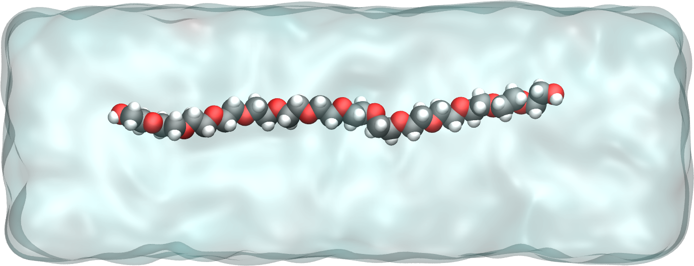
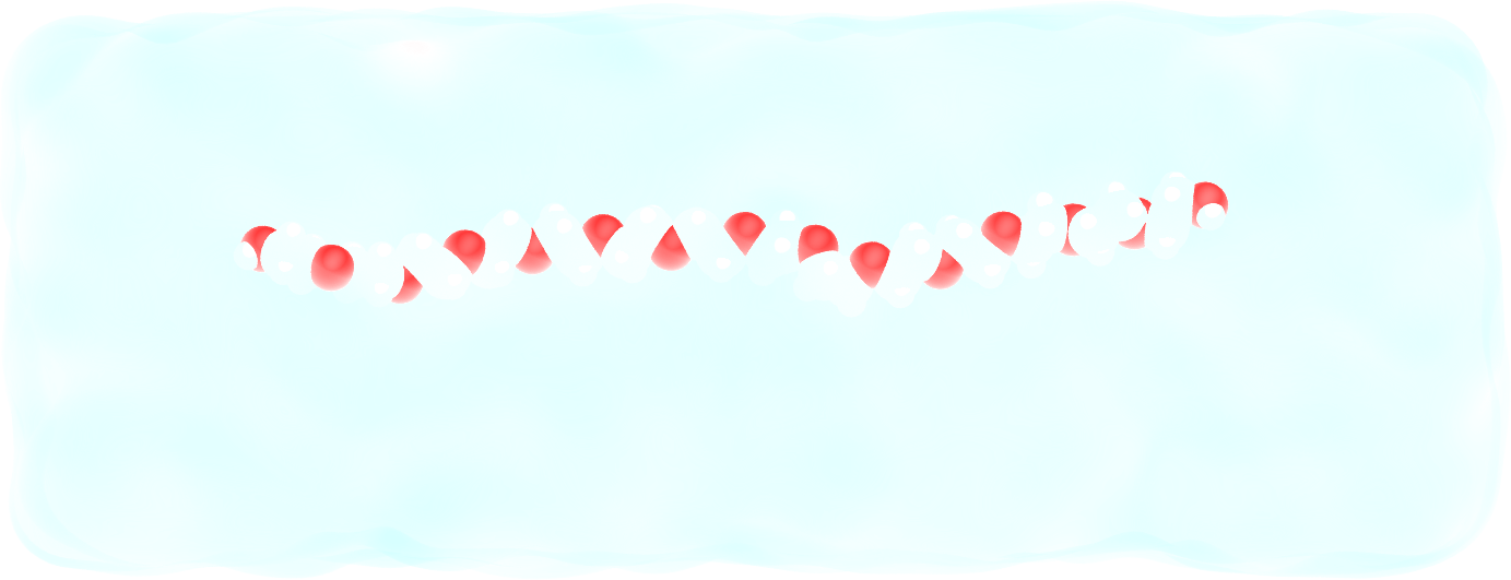
Figure: PEG molecule stretched along the \(x\) direction in water.

Run the pull.lmp file using LAMMPS. From the generated images of the system, you should observe that the PEG molecule eventually aligns in the direction of the applied force. The evolutions of the radius of gyration over time indicates that the PEG quickly adjusts to the external force. Additionally, from the values of the dihedral angles printed in the pull.dat file, you can create a histogram of dihedral angles for a specific type. For example, the angle \(\phi\) for dihedrals of type 1 (C-C-OE-C) is shown below.

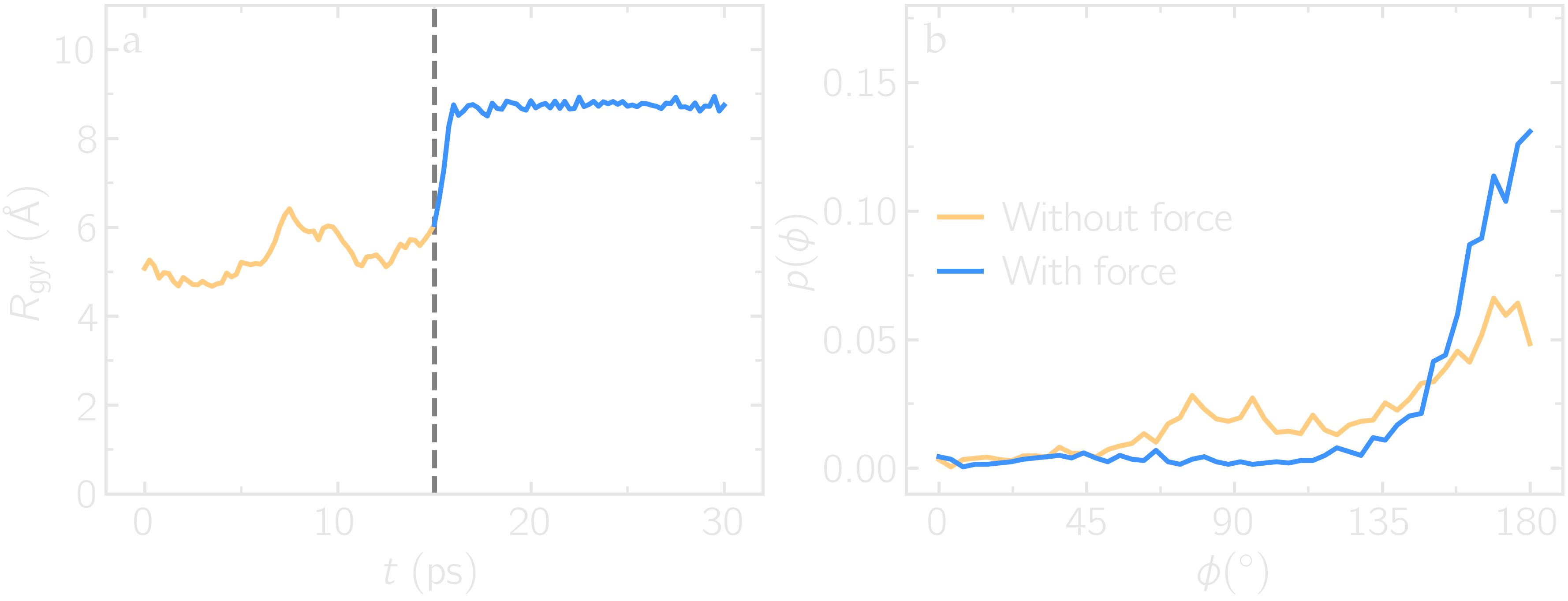
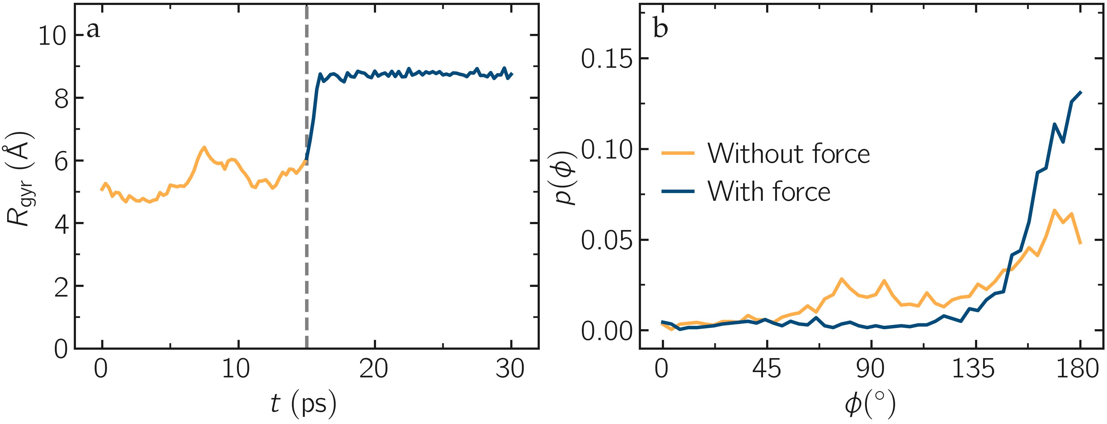
Figure: a) Evolution of the radius of gyration \(R_\text{gyr}\) of the PEG molecule, with the force applied starting at \(t = 15\,\text{ps}\). b) Histograms of the dihedral angles of type 1 in the absence (orange) and in the presence (blue) of the applied force.

Tip: using external visualization tools

Trajectories can be visualized using external tools such as VMD or OVITO [12, 13]. To do so, the IDs and positions of the atoms must be regularly written to a file during the simulation. This can be accomplished by adding a dump command to the input file. For instance, create a duplicate of pull.lmp and name it pull-with-tip.lmp. Then, replace the existing dump and dump_modify commands with:

dump mydmp all atom 1000 pull.lammpstrj

Running the pull-with-tip.lmp file using LAMMPS will generate a trajectory file named pull.lammpstrj, which can be opened in OVITO or VMD.

Note

Since the trajectory dump file does not contain information about topology and elements, it is usually preferred to first write out a data file and import it directly (in the case of OVITO) or convert it to a PSF file (for VMD). This allows the topology to be loaded before adding the trajectory file to it. When using LAMMPS–GUI, this process can be automated through the View in OVITO or View in VMD options in the Run menu. Afterwards only the trajectory dump needs to be added.

Cite

You can access the input scripts and data files that are used in these tutorials from a dedicated Github repository. This repository also contains the full solutions to the exercises.

Going further with exercises

Extract the radial distribution function

Extract the radial distribution functions (RDF or \(g(r)\)) between the oxygen atom of the water molecules and the oxygen atom from the PEG molecule. Compare the rdf before and after the force is applied to the PEG.

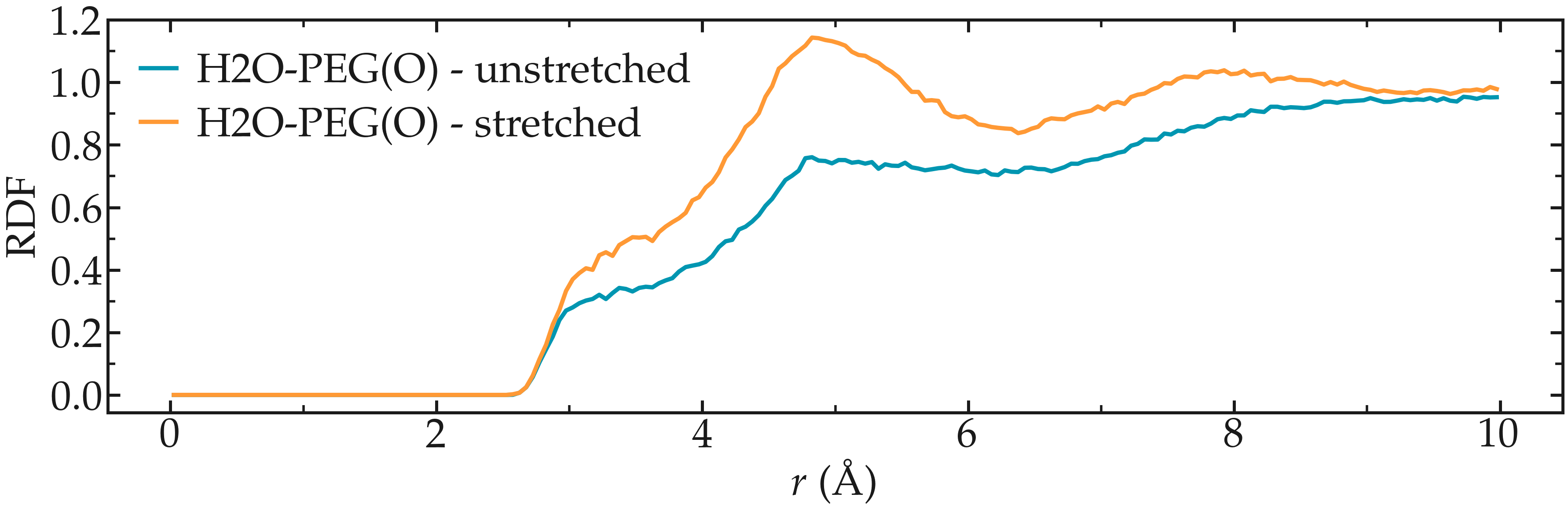
Figure: Radial distribution function between the oxygen atoms of water, as well as between the oxygen atoms of water and the oxygen atoms of the PEG molecule.

Note the difference in the structure of the water before and after the PEG molecule is stretched. This effect is described in the 2017 publication by Liese et al. [26].

Add salt to the system

Realistic systems usually contain ions. Let us add some \(\text{Na}^+\) and \(\text{Cl}^-\) ions to our current PEG-water system.

Add some \(\text{Na}^+\) and \(\text{Cl}^-\) ions to the mixture using the method of your choice. \(\text{Na}^+\) ions are characterised by their mass \(m = 22.98\,\text{g/mol}\), their charge \(q = +1\,e\), and Lennard-Jones parameters, \(\epsilon = 0.0469\,\text{kcal/mol}\) and \(\sigma = 0.243\,\text{nm}\), and \(\text{Cl}^-\) ions by their mass \(m = 35.453\,\text{g/mol}\), charge \(q = -1\,e\) and Lennard-Jones parameters, \(\epsilon = 0.15\,\text{kcal/mol}\), and \(\sigma = 0.4045\,\text{nm}\).

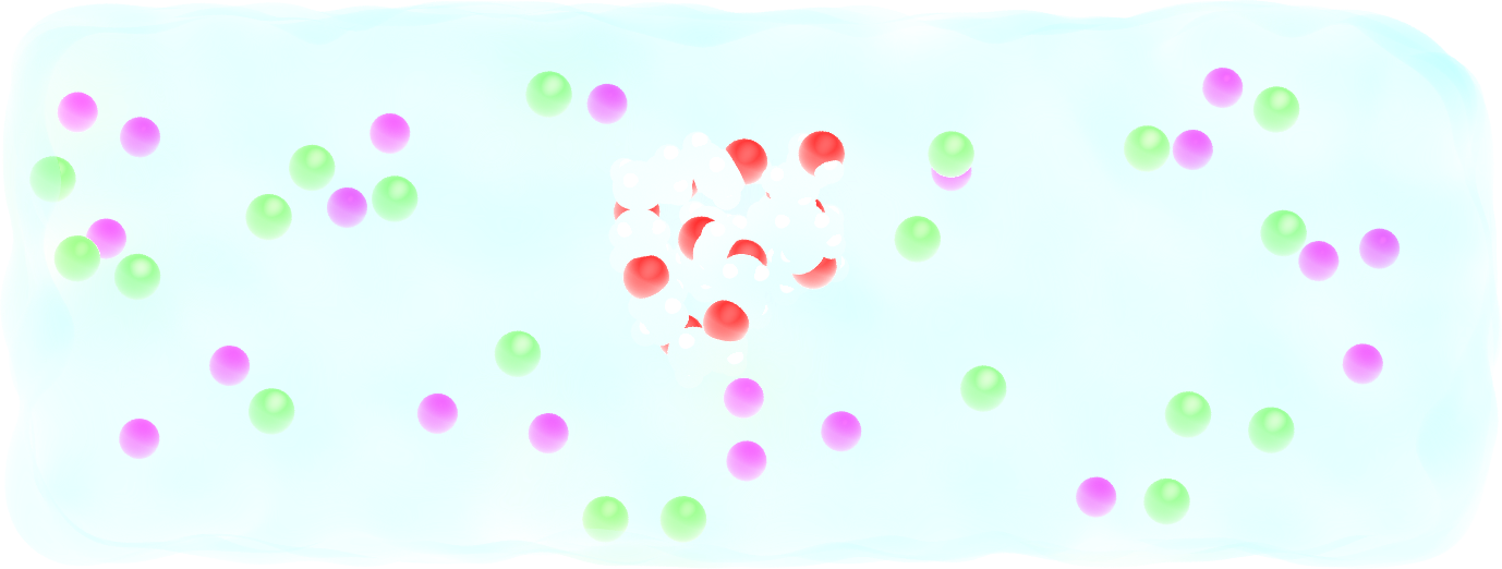
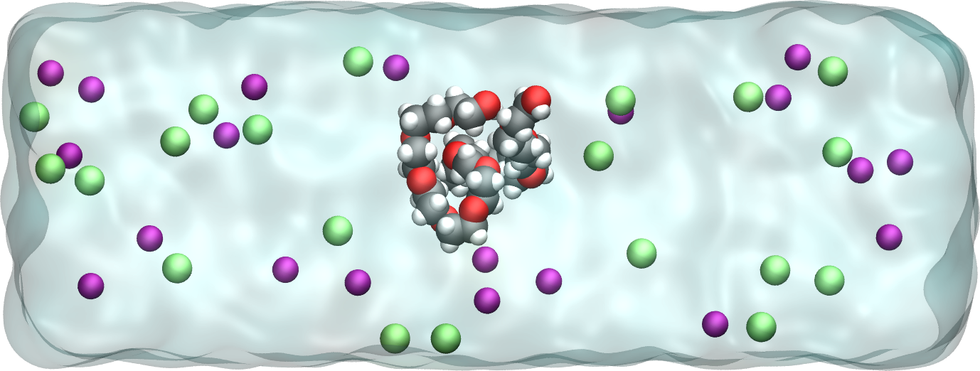
Figure: A PEG molecule in the electrolyte with \(\text{Na}^+\) ions in purple and \(\text{Cl}^-\) ions in cyan.

Evaluate the deformation of the PEG

Once the PEG is fully stretched, its structure differs from the unstretched case. The deformation can be probed by extracting the typical intra-molecular parameters, such as the typical angles of the dihedrals.

Extract the histograms of the angular distribution of the PEG dihedrals in the absence and the presence of stretching.

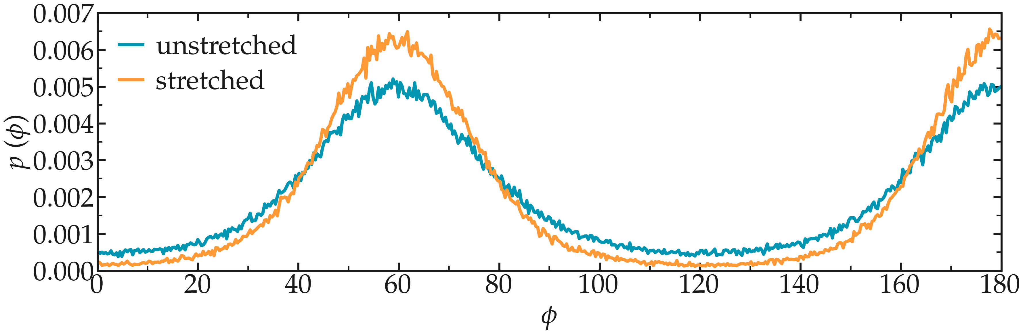
Figure: Probability distribution for the dihedral angle \(\phi\), for a stretched and for an unstretched PEG molecule.