Reactive Molecular Dynamics

Modeling reaction using the REACTER protocol

The goal of this tutorial is to create a model of a carbon nanotube (CNT) embedded in a polymer melt composed of polystyrene (PS). The REACTER protocol is used to simulate the polymerization of styrene monomers, and the polymerization reaction is tracked over time [55, 56, 57]. In contrast to AIREBO Pulling on a carbon nanotube and ReaxFF Reactive silicon dioxide, the REACTER protocol relies on the use of a classical force field.

If you are completely new to LAMMPS, we recommend that you follow this tutorial on a simple Lennard-Jones fluid first.

Cite

If you find these tutorials useful, you can cite A Set of Tutorials for the LAMMPS Simulation Package by Simon Gravelle, Jacob R. Gissinger, and Axel Kohlmeyer (2025) [14]. You can access the full paper on arXiv.

This tutorial is compatible with the 29Aug2024 (update 2) LAMMPS version.

Creating the system

To begin this tutorial, select Start Tutorial 8 from the Tutorials menu of LAMMPS–GUI and follow the instructions. The editor should display the following content corresponding to mixing.lmp:

units real
boundary p p p
atom_style full

kspace_style pppm 1.0e-5
pair_style lj/class2/coul/long 8.5
angle_style class2
bond_style class2
dihedral_style class2
improper_style class2

pair_modify tail yes mix sixthpower
special_bonds lj/coul 0 0 1

The class2 styles compute a 6/9 Lennard-Jones potential [58]. The class2 bond, angle, dihedral, and improper styles are used as well, see the documentation for a description of their respective potentials. The mix sixthpower imposes the following mixing rule for the calculation of the cross coefficients:

\[\sigma_{ij} = 2^{-1/6} (\sigma^6_i+\sigma_j^6)^{1/6},\]

and

\[\epsilon_{ij} = \dfrac{2 \sqrt{\epsilon_i \epsilon_j} \sigma^3_i \sigma^3_j}{\sigma^6_i+\sigma_j^6}.\]

Let us read the CNT.data file, which contains a periodic single-walled CNT. Add the following line to mixing.lmp:

read_data CNT.data extra/special/per/atom 20

The CNT is approximately \(1.1~\text{nm}\) in diameter and \(1.6\,\text{nm}\) in length, oriented along the \(x\)-axis. The simulation box is initially 12.0 nm in the two other dimensions before densification, making it straightforward to fill the box with styrene. To add 200 styrene molecules to the simulation box, we will use the styrene.mol molecule template file. Include the following commands to mixing.lmp:

molecule styrene styrene.mol
create_atoms 0 random 200 8305 NULL overlap 2.75 maxtry 500 mol styrene 7687

Finally, let us use the minimize command to reduce the potential energy of the system:

minimize 1.0e-4 1.0e-6 100 1000
reset_timestep 0

Then, let us densify the system to a target value of \(0.9~\text{g/cm}^3\) by manually shrinking the simulation box at a constant rate. The dimension parallel to the CNT axis is maintained fixed because the CNT is periodic in that direction. Add the following commands to mixing.lmp:

velocity all create 530 9845 dist gaussian rot yes
fix mynvt all nvt temp 530 530 100

fix mydef all deform 1 y erate -0.0001 z erate -0.0001
variable rho equal density
fix myhal all halt 10 v_rho > 0.9 error continue

thermo 200
thermo_style custom step temp pe etotal press density

run 9000

The fix halt command is used to stop the box shrinkage once the target density is reached.

For the next stage of the simulation, we will use dump image to output images every 200 steps:

dump viz all image 200 myimage-*.ppm type type shiny 0.1 box no 0.01 size 1000 1000 view 90 0 zoom 1.8 fsaa yes bond atom 0.5
dump_modify viz backcolor white acolor cp gray acolor c=1 gray acolor c= gray acolor c1 deeppink &
    acolor c2 deeppink acolor c3 deeppink adiam cp 0.3 adiam c=1 0.3 adiam c= 0.3 adiam c1 0.3 &
    adiam c2 0.3 adiam c3 0.3 acolor hc white adiam hc 0.15

For the following \(10~\text{ps}\), let us equilibrate the densified system in the constant-volume ensemble, and write the final state of the system in a file named mixing.data:

unfix mydef
unfix myhal
reset_timestep 0

group CNT molecule 1
fix myrec CNT recenter NULL 0 0 units box shift all

run 10000

write_data mixing.data

For visualization purposes, the atoms from the CNT group is moved to the center of the box using fix recenter. As the time progresses, the system density, \(\rho\), gradually converges toward the target value of \(0.8\),g/cm:math:^3. Meanwhile, the total energy of the system initially evolves rapidly, reflecting the densification process, and then eventually stabilizes.

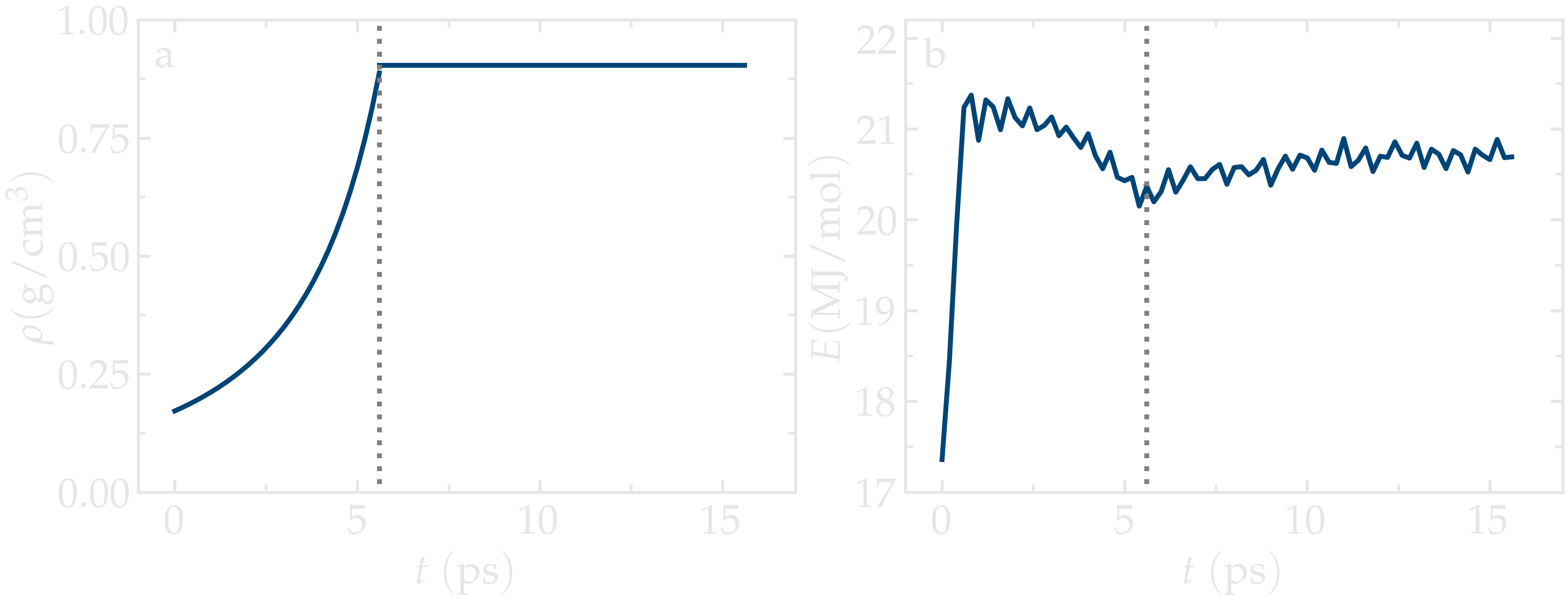
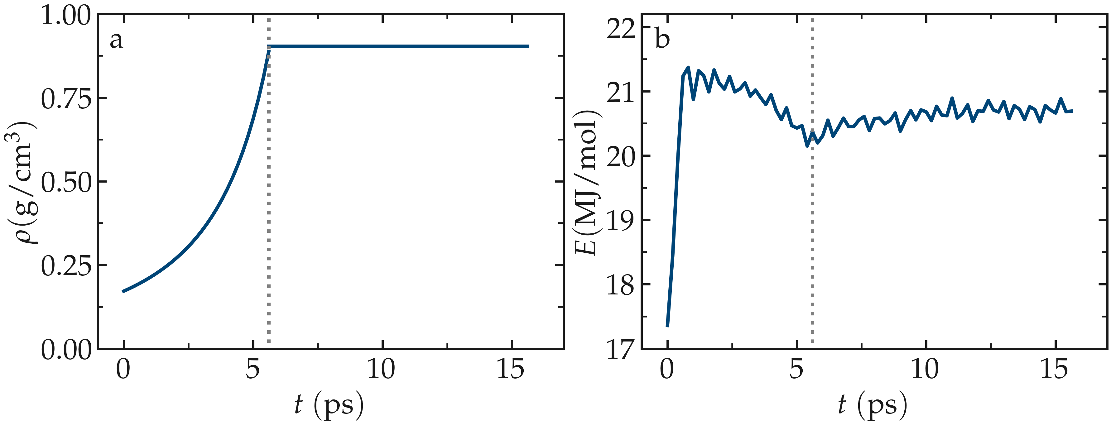
Figure: a) Evolution of the density, \(\rho\), as a function of the time, \(t\), during equilibration of the system. b) Evolution of the total energy, \(E\), of the system. The vertical dashed lines mark the transition between the different phases of the simulation.

Reaction templates

The REACTER protocol enables the modeling of chemical reactions using classical force fields. The user must provide a molecule template for the reactants, a molecule template for the products, and a reaction map file that provides an atom mapping between the two templates. The reaction map file also includes additional information, such as which atoms act as initiators for the reaction and which serve as edge atoms to connect the rest of a long polymer chain in the simulation.

There are three reactions to define: (1) the polymerization of two styrene monomers, (2) the addition of a styrene monomer to the end of a growing polymer chain, and (3) the linking of two polymer chains. Download the three files associated with each reaction. The first reaction uses the prefix M-M for the pre-reaction template, post-reaction template, and reaction map file:

• M-M_pre.mol,

• M-M_post.mol,

• M-M.rxnmap.

The second reaction uses the prefix M-P,

• M-P_pre.mol,

• M-P_post.mol,

• M-P.rxnmap.

The third reaction uses the prefix P-P,

• P-P_pre.mol,

• P-P_post.mol,

• P-P.rxnmap.

Here, the file names for each reaction use the abbreviation M for monomer and P for polymer.

Simulating the reaction

The first step, before simulating the reaction, is to import the previously generated configuration. Open the file named polymerize.lmp, which should contain the following lines:

units real
boundary p p p
atom_style full

kspace_style pppm 1.0e-5
pair_style lj/class2/coul/long 8.5
angle_style class2
bond_style class2
dihedral_style class2
improper_style class2

pair_modify tail yes mix sixthpower
special_bonds lj/coul 0 0 1

read_data mixing.data extra/bond/per/atom 5  extra/angle/per/atom 15 extra/dihedral/per/atom 15 extra/improper/per/atom 25 extra/special/per/atom 25

Here, the read_data command is used to import the previously generated mixing.data file. All other commands have been introduced in earlier parts of the tutorial.

Then, let us import all six molecules templates using the molecule command:

molecule mol1 M-M_pre.mol
molecule mol2 M-M_post.mol
molecule mol3 M-P_pre.mol
molecule mol4 M-P_post.mol
molecule mol5 P-P_pre.mol
molecule mol6 P-P_post.mol

In order to follow the evolution of the reaction with time, let us generate images of the system using dump image:

dump viz all image 200 myimage-*.ppm type type shiny 0.1 box no 0.01 size 1000 1000 view 90 0 zoom 1.8 fsaa yes bond atom 0.5
dump_modify viz backcolor white acolor cp gray acolor c=1 gray acolor c= gray acolor c1 deeppink acolor c2 gray acolor c3 deeppink &
    adiam cp 0.3 adiam c=1 0.3 adiam c= 0.3 adiam c1 0.3 adiam c2 0.3 adiam c3 0.3 acolor hc white adiam hc 0.15

Let us use fix bond/react by adding the following line to polymerize.lmp:

fix rxn all bond/react stabilization yes statted_grp 0.03 react R1 all 1 0 3.0 mol1 mol2 M-M.rxnmap &
    react R2 all 1 0 3.0 mol3 mol4 M-P.rxnmap react R3 all 1 0 5.0 mol5 mol6 P-P.rxnmap

With the stabilization keyword, the bond/react command will stabilize the atoms involved in the reaction using the nve/limit command with a maximum displacement of \(0.03\,\text{Å}\). By default, each reaction is stabilized for 60 time steps. Each react keyword corresponds to a reaction, e.g., a transformation of mol1 into mol2 based on the atom map M-M.rxnmap. Implementation details about each reaction, such as the reaction distance cutoffs and the frequency with which to search for reaction sties, are also specified in this command.

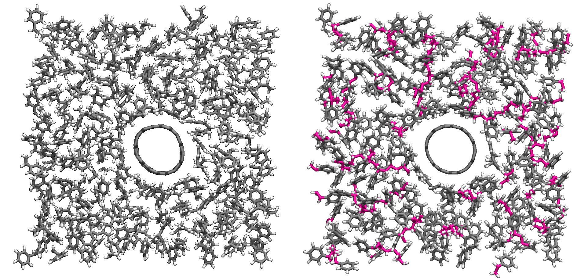
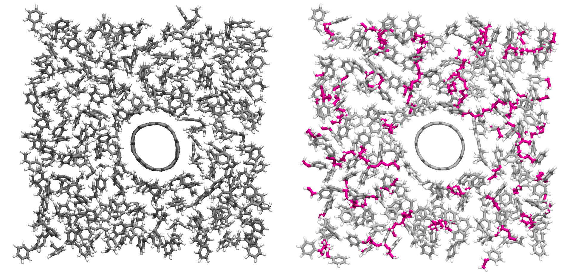
Figure: Initial (left) and final (right) configuration. The atoms from the formed polymer named c1, c2, and c3 are colored in pink.

Note

The command fix bond/react creates several groups of atoms that are dynamically updated to track which atoms are being stabilized and which atoms are undergoing dynamics with the system-wide time integrator (here, fix nvt). When reaction stabilization is employed, there should not be a time integrator acting on the group all. Instead, the group of atoms not currently undergoing stabilization is named by appending _REACT to the user-provided prefix.

Add the following commands to polymerize.lmp to operate in the NVT ensemble while ensuring that the CNT remains centered in the simulation box:

fix mynvt statted_grp_REACT nvt temp 530 530 100
group CNT molecule 1 2 3
fix myrec CNT recenter NULL 0 0 shift all

thermo 1000
thermo_style custom step temp press density f_rxn[*]

run 25000

Here, the thermo custom command is used to print the cumulative reaction counts from fix rxn. Run the simulation using LAMMPS. As the simulation progresses, polymer chains are observed forming. During this reaction process, the temperature of the system remains well-controlled, while the number of reactions, \(N_r\), increases with time.

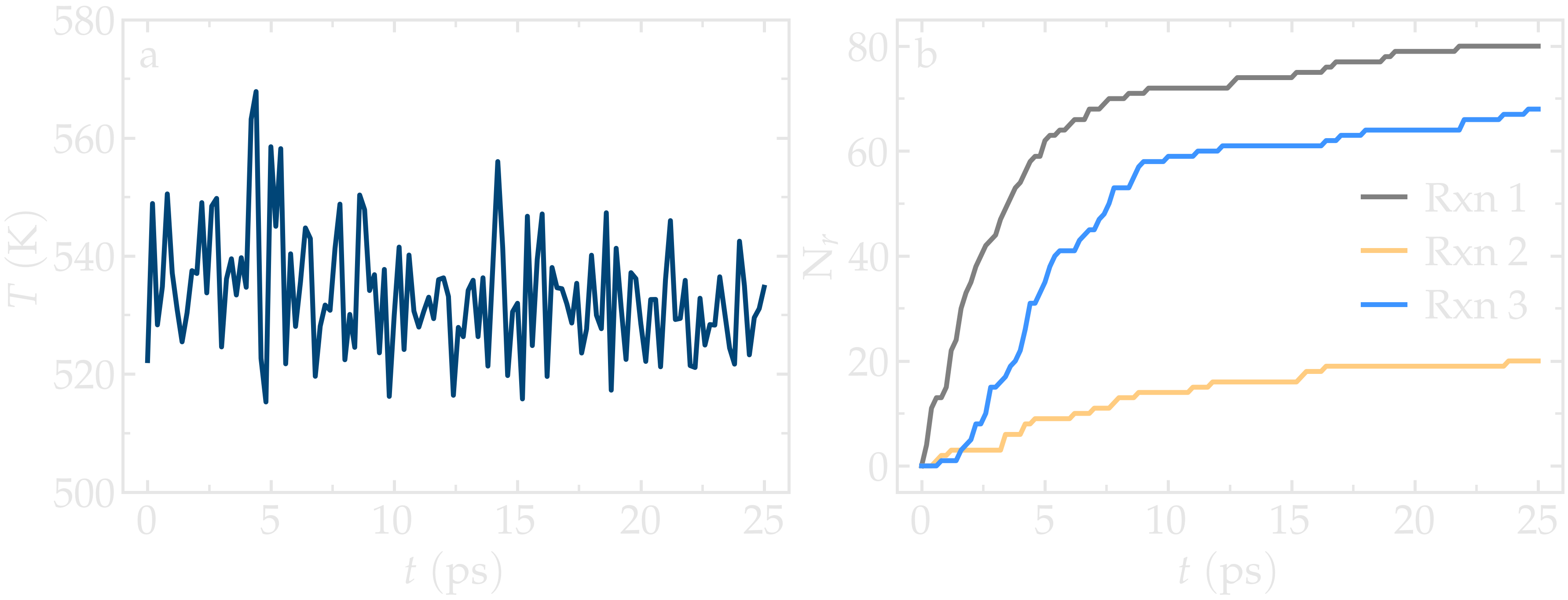
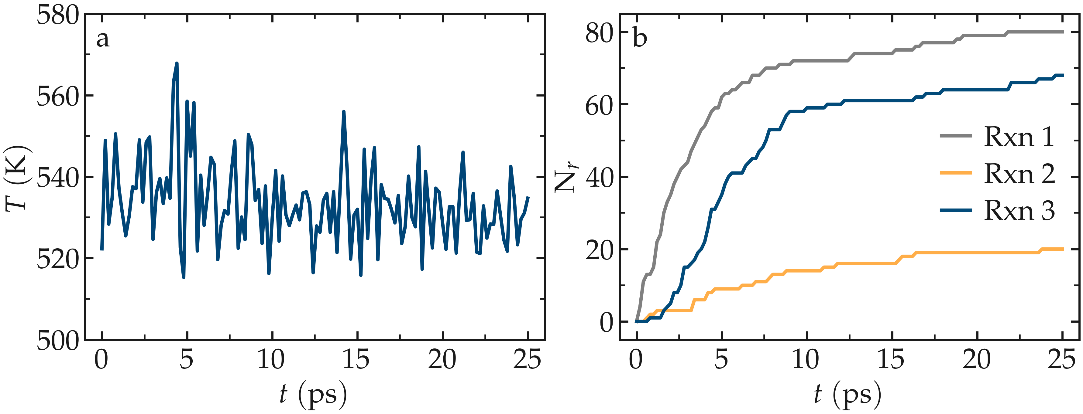
Figure: a) Evolution of the system temperature, \(T\), as a function of the time, \(t\), during the polymerization step. b) Evolution of the three reaction counts, corresponding respectively to the polymerization of two styrene monomers (Rxn 1), the addition of a styrene monomer to the end of a growing polymer chain (Rxn 2), and to the linking of two polymer chains (Rxn 3).

Cite

You can access the input scripts and data files that are used in these tutorials from a dedicated Github repository. This repository also contains the full solutions to the exercises.