Nanosheared electrolyte

Aqueous NaCl solution sheared by two walls

The objective of this tutorial is to simulate an electrolyte nanoconfined and sheared between two walls. The density and velocity profiles of the fluid in the direction normal to the walls are extracted to highlight the effect of confining a fluid on its local properties. This tutorial demonstrates key concepts of combining a fluid and a solid in the same simulation. A major difference from the previous tutorial, Polymer in water, is that here a rigid four-point water model named TIP4P/2005 is used [4].

Note

Four-point water models such as TIP4P/2005 are widely used as they offer a good compromise between accuracy and computational cost [33].

If you are completely new to LAMMPS, we recommend that you follow this tutorial on a simple Lennard-Jones fluid first.

Cite

If you find these tutorials useful, you can cite A Set of Tutorials for the LAMMPS Simulation Package by Simon Gravelle, Jacob R. Gissinger, and Axel Kohlmeyer (2025) [14]. You can access the full paper on arXiv.

This tutorial is compatible with the 29Aug2024 (update 2) LAMMPS version.

System preparation

The fluid and walls must first be generated, followed by equilibration at the desired temperature and pressure.

System generation

Create a folder if needed and place the initial input file, create.lmp, into it. Then, open the file in a text editor of your choice, and copy the following into it:

boundary p p f
units real
atom_style full
bond_style harmonic
angle_style harmonic
pair_style lj/cut/tip4p/long O H O-H H-O-H 0.1546 12.0
kspace_style pppm/tip4p 1.0e-5
kspace_modify slab 3.0

If you are using LAMMPS-GUI

To begin this tutorial, select Start Tutorial 4 from the Tutorials menu of LAMMPS–GUI and follow the instructions. The editor should display the following content corresponding to create.lmp

These lines are used to define the most basic parameters, including the atom, bond, and angle styles, as well as interaction potential. Here, lj/cut/tip4p/long imposes a Lennard-Jones potential with a cut-off at \(12\,\text{Å}\) and a long-range Coulomb potential.

So far, the commands are relatively similar to those in the previous tutorial, Polymer in water, with two major differences: the use of lj/cut/tip4p/long instead of lj/cut/coul/long, and pppm/tip4p instead of pppm. When using lj/cut/tip4p/long and pppm/tip4p, the interactions resemble the conventional Lennard-Jones and Coulomb interactions, except that they are specifically designed for the four-point water model. As a result, LAMMPS automatically creates a four-point water molecule, assigning type O atoms as oxygen and type H atoms as hydrogen. The fourth massless atom (M) of the TIP4P water molecule does not have to be defined explicitly, and the value of \(0.1546\,\text{Å}\) corresponds to the O-M distance of the TIP4P-2005 water model [4]. All other atoms in the simulation are treated as usual, with long-range Coulomb interactions. Another novelty, here, is the use of kspace modify slab 3.0 that is combined with the non-periodic boundaries along the \(z\) coordinate: boundary p p f. With the slab option, the system is treated as periodical along \(z\), but with an empty volume inserted between the periodic images of the slab, and the interactions along \(z\) effectively turned off.

Let us create the box and the label maps by adding the following lines to create.lmp:

lattice fcc 4.04
region box block -3 3 -3 3 -5 5
create_box 5 box bond/types 1 angle/types 1 extra/bond/per/atom 2 extra/angle/per/atom 1 &
    extra/special/per/atom 2
labelmap atom 1 O 2 H 3 Na+ 4 Cl- 5 WALL
labelmap bond 1 O-H
labelmap angle 1 H-O-H

The lattice command defines the unit cell. Here, the face-centered cubic (fcc) lattice with a scale factor of 4.04 has been chosen for the future positioning of the atoms of the walls. The region command defines a geometric region of space. By choosing \(\text{xlo}=-3\) and \(\text{xlo}=3\), and because we have previously chosen a lattice with a scale factor of 4.04, the region box extends from \(-12.12~\text{Å}\) to \(12.12~\text{Å}\) along the \(x\) direction. The create_box command creates a simulation box with 5 types of atoms: the oxygen and hydrogen of the water molecules, the two ions (\(\text{Na}^+\), \(\text{Cl}^-\)), and the atoms from the walls. The simulation contains 1 type of bond and 1 type of angle (both required by the water molecules). The parameters for these bond and angle constraints will be given later. The extra (...) keywords are for memory allocation. Finally, the labelmap commands assign alphanumeric type labels to each numeric atom type, bond type, and angle type.

Now, we can add atoms to the system. First, let us create two sub-regions corresponding respectively to the two solid walls, and create a larger region from the union of the two regions. Then, let us create atoms of type WALL within the two regions. Add the following lines to create.lmp:

region rbotwall block -3 3 -3 3 -4 -3
region rtopwall block -3 3 -3 3 3 4
region rwall union 2 rbotwall rtopwall
create_atoms WALL region rwall

Atoms will be placed in the positions of the previously defined lattice, thus forming fcc solids.

To add the water molecules, the molecule template called water.mol must be located next to create.lmp. The template contains all the necessary information concerning the water molecule, such as atom positions, bonds, and angles. Add the following lines to create.lmp:

region rliquid block INF INF INF INF -2 2
molecule h2omol water.mol
create_atoms 0 region rliquid mol h2omol 482793

Within the last three lines, a region named rliquid is created based on the last defined lattice, fcc 4.04. rliquid will be used for depositing the water molecules. The molecule command opens up the molecule template called water.mol, and names the associated molecule h2omol. The new molecules are placed on the fcc 4.04 lattice by the create_atoms command. The first parameter is 0, meaning that the atom IDs from the water.mol file will be used. The number 482793 is a seed that is required by LAMMPS, it can be any positive integer.

Finally, let us create 30 ions (15 \(\text{Na}^+\) and 15 \(\text{Cl}^-\)) in between the water molecules, by adding the following commands to create.lmp:

create_atoms Na+ random 15 5802 rliquid overlap 0.3 maxtry 500
create_atoms Cl- random 15 9012 rliquid overlap 0.3 maxtry 500
set type Na+ charge 1
set type Cl- charge -1

Each create_atoms command will add 15 ions at random positions within the rliquid region, ensuring that there is no overlap with existing molecules. Feel free to increase or decrease the salt concentration by changing the number of desired ions. To keep the system charge neutral, always insert the same number of \(\text{Na}^+\) and \(\text{Cl}^-\), unless there are other charges in the system. The charges of the newly added ions are specified by the two set commands.

Before starting the simulation, we need to define the parameters of the simulation: the mass of the 5 atom types (O, H, \(\text{Na}^+\), \(\text{Cl}^-\), and wall), the pairwise interaction parameters (in this case, for the Lennard-Jones potential), and the bond and angle parameters. Copy the following lines into create.lmp:

include parameters.inc
include groups.inc

Both parameters.inc and groups.inc files must be located next to create.lmp. The parameters.inc file contains the masses, as follows:

mass O 15.9994
mass H 1.008
mass Na+ 22.990
mass Cl- 35.453
mass WALL 26.9815

Each mass command assigns a mass in g/mol to an atom type. The parameters.inc file also contains the pair coefficients:

pair_coeff O O 0.185199 3.1589
pair_coeff H H 0.0 1.0
pair_coeff Na+ Na+ 0.04690 2.4299
pair_coeff Cl- Cl- 0.1500 4.04470
pair_coeff WALL WALL 11.697 2.574
pair_coeff O WALL 0.4 2.86645

Each pair_coeff assigns the depth of the LJ potential (in kcal/mol), and the distance (in Ångströms) at which the particle-particle potential energy is 0. As noted in previous tutorials, with the important exception of pair_coeff O WALL, pairwise interactions were only assigned between atoms of identical types. By default, LAMMPS calculates the pair coefficients for the interactions between atoms of different types (i and j) by using geometric average: \(\epsilon_{ij} = (\epsilon_{ii} + \epsilon_{jj})/2\), \(\sigma_{ij} = (\sigma_{ii} + \sigma_{jj})/2\). However, if the default value of \(5.941\,\text{kcal/mol}\) was used for \(\epsilon_\text{1-5}\), the solid walls would be extremely hydrophilic, causing the water molecules to form dense layers. As a comparison, the water-water energy \(\epsilon_\text{1-1}\) is only \(0.185199\,\text{kcal/mol}\). Therefore, to make the walls less hydrophilic, the value of \(\epsilon_\text{O-WALL}\) was reduced.

Finally, the parameters.inc file contains the following two lines:

bond_coeff O-H 0 0.9572
angle_coeff H-O-H 0 104.52

The bond_coeff command, used here for the O-H bond of the water molecule, sets both the spring constant of the harmonic potential and the equilibrium bond distance of \(0.9572~\text{Å}\). The constant can be 0 for a rigid water molecule because the SHAKE algorithm will maintain the rigid structure of the water molecule (see below) [34, 35]. Similarly, the angle_coeff command for the H-O-H angle of the water molecule sets the force constant of the angular harmonic potential to 0 and the equilibrium angle to \(104.52^\circ\).

Alongside parameters.inc, the groups.inc file contains several group commands to selects atoms based on their types:

group H2O type O H
group Na type Na+
group Cl type Cl-
group ions union Na Cl
group fluid union H2O ions

The groups.inc file also defines the walltop and wallbot groups, which contain the WALL atoms located in the \(z > 0\) and \(z < 0\) regions, respectively:

group wall type WALL
region rtop block INF INF INF INF 0 INF
region rbot block INF INF INF INF INF 0
group top region rtop
group bot region rbot
group walltop intersect wall top
group wallbot intersect wall bot

Currently, the fluid density between the two walls is slightly too high. To avoid excessive pressure, let us add the following lines into create.lmp to delete about \(15~\%\) of the water molecules:

delete_atoms random fraction 0.15 yes H2O NULL 482793 mol yes

To create an image of the system, add the following dump image into create.lmp:

dump mydmp all image 200 myimage-*.ppm type type shiny 0.1 box no 0.01 view 90 0 zoom 1.8
dump_modify mydmp backcolor white acolor O red adiam O 2 acolor H white adiam H 1 &
    acolor Na+ blue adiam Na+ 2.5 acolor Cl- cyan adiam Cl- 3 acolor WALL gray adiam WALL 3

Finally, add the following lines into create.lmp:

run 0

write_data create.data nocoeff

The run 0 command runs the simulation for 0 steps, which is sufficient for creating the system and saving its state. The write_data command generates a file called system.data containing the information required to restart the simulation from the final configuration produced by this input file. With the nocoeff option, the parameters from the force field are not included in the .data file. Run the create.lmp file using LAMMPS, and a file named create.data will be created alongside create.lmp.

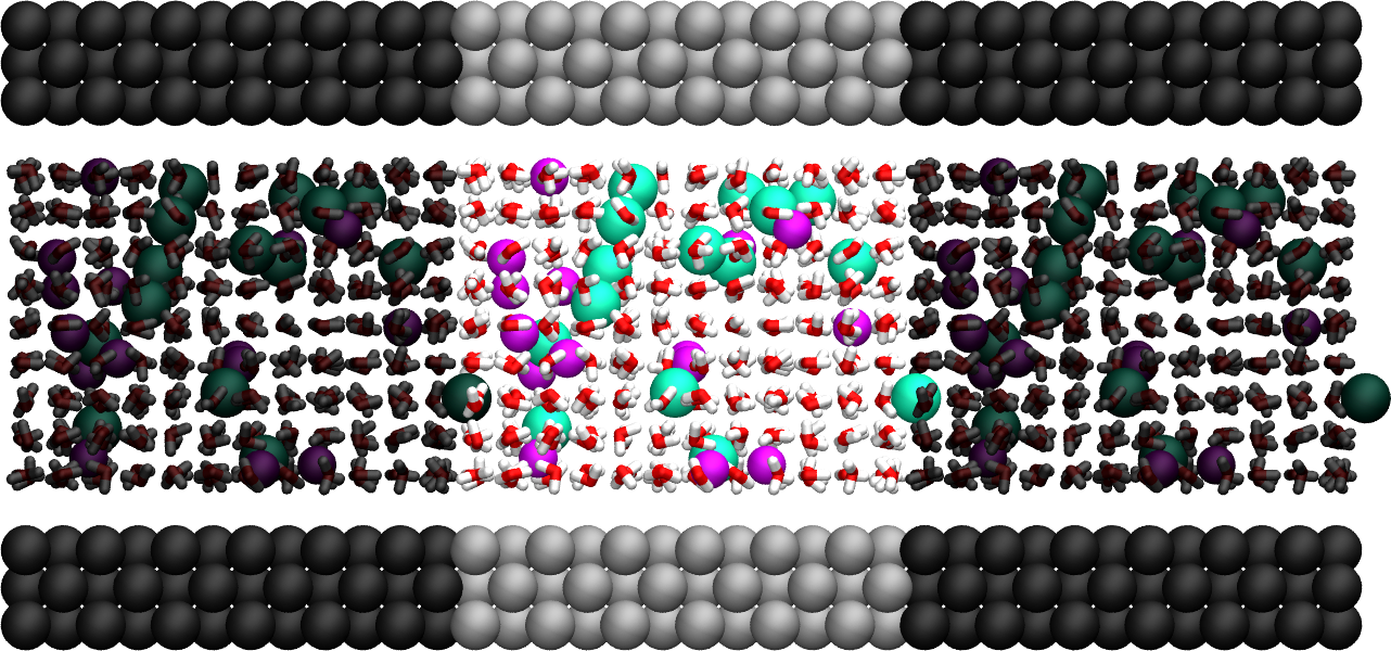
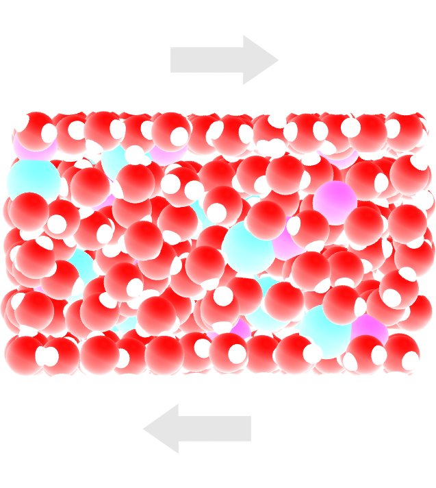
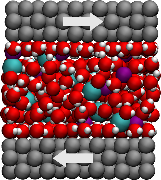
Figure: Side view of the system. Periodic images are represented in darker colors. Water molecules are in red and white, \(\text{Na}^+\) ions in pink, \(\text{Cl}^-\) ions in lime, and wall atoms in gray. Note the absence of atomic defect at the cell boundaries.

Energy minimization

Let us move the atoms and place them in more energetically favorable positions before starting the actual molecular dynamics simulation.

If you are using LAMMPS-GUI

Open the equilibrate.lmp file that was downloaded alongside create.lmp during the tutorial setup.

Create a new file, equilibrate.lmp, and copy the following into it:

boundary p p f
units real
atom_style full
bond_style harmonic
angle_style harmonic
pair_style lj/cut/tip4p/long O H O-H H-O-H 0.1546 12.0
kspace_style pppm/tip4p 1.0e-5
kspace_modify slab 3.0

read_data create.data

include parameters.inc
include groups.inc

The only difference from the previous input is that, instead of creating a new box and new atoms, we open the previously created create.data file.

Now, let us use the SHAKE algorithm to maintain the shape of the water molecules [34, 35].

fix myshk H2O shake 1.0e-5 200 0 b O-H a H-O-H kbond 2000

Here the SHAKE algorithm applies to the O-H bond and the H-O-H angle of the water molecules. The kbond keyword specifies the force constant that will be used to apply a restraint force when used during minimization. This last keyword is important here, because the spring constants of the rigid water molecules were set to 0 (see the parameters.inc file).

Let us also create images of the system and control the printing of thermodynamic outputs by adding the following lines to equilibrate.lmp:

dump mydmp all image 1 myimage-*.ppm type type shiny 0.1 box no 0.01 view 90 0 zoom 1.8
dump_modify mydmp backcolor white acolor O red adiam O 2 acolor H white adiam H 1 &
    acolor Na+ blue adiam Na+ 2.5 acolor Cl- cyan adiam Cl- 3 acolor WALL gray adiam WALL 3

thermo 1
thermo_style custom step temp etotal press

Let us perform an energy minization by adding the following lines to equilibrate.lmp:

minimize 1.0e-6 1.0e-6 1000 1000
reset_timestep 0

When running the equilibrate.lmp file with LAMMPS, you should observe that the total energy of the system is initially very high but rapidly decreases. From the generated images of the system, you will notice that the atoms and molecules are moving to adopt more favorable positions.

System equilibration

Let us equilibrate further the entire system by letting both fluid and piston relax at ambient temperature. Here, the commands are written within the same equilibrate.lmp file, right after the reset_timestep command.

Let us update the positions of all the atoms and use a Nosé-Hoover thermostat. Add the following lines to equilibrate.lmp:

fix mynvt all nvt temp 300 300 100
fix myshk H2O shake 1.0e-5 200 0 b O-H a H-O-H
fix myrct all recenter NULL NULL 0
timestep 1.0

As mentioned previously, the fix recenter does not influence the dynamics, but will keep the system in the center of the box, which makes the visualization easier. Then, add the following lines into equilibrate.lmp for the trajectory visualization:

undump mydmp
dump mydmp all image 250 myimage-*.ppm type type shiny 0.1 box no 0.01 view 90 0 zoom 1.8
dump_modify mydmp backcolor white acolor O red adiam O 2 acolor H white adiam H 1 &
    acolor Na+ blue adiam Na+ 2.5 acolor Cl- cyan adiam Cl- 3 acolor WALL gray adiam WALL 3

The undump command is used to cancel the previous dump command. Then, a new dump command with a larger dumping period is used.

To monitor the system equilibration, let us print the distance between the two walls. Add the following lines to equilibrate.lmp:

variable walltopz equal xcm(walltop,z)
variable wallbotz equal xcm(wallbot,z)
variable deltaz equal v_walltopz-v_wallbotz

thermo 250
thermo_style custom step temp etotal press v_deltaz

The first two variables extract the centers of mass of the two walls. The deltaz variable is then used to calculate the difference between the two variables walltopz and wallbotz, i.e. the distance between the two centers of mass of the walls.

Finally, let us run the simulation for 30 ps by adding a run command to equilibrate.lmp:

run 30000

write_data equilibrate.data nocoeff

Run the equilibrate.lmp file using LAMMPS. Both the pressure and the distance between the two walls show oscillations at the start of the simulation but eventually stabilize at their equilibrium values toward the end of the simulation.

Note

Note that it is generally recommended to run a longer equilibration. In this case, the slowest process in the system is likely ionic diffusion. Therefore, the equilibration period should, in principle, exceed the time required for the ions to diffuse across the size of the pore, i.e. \(H_\text{pore}^2/D_\text{ions}\). Using \(H_\text{pore} \approx 1.2~\text{nm}\) as the final pore size and \(D_\text{ions} \approx 1.5 \cdot 10^{-9}~\text{m}^2/\text{s}\) as the typical diffusion coefficient for sodium chloride in water at room temperature [36], one finds that the equilibration should be on the order of one nanosecond.

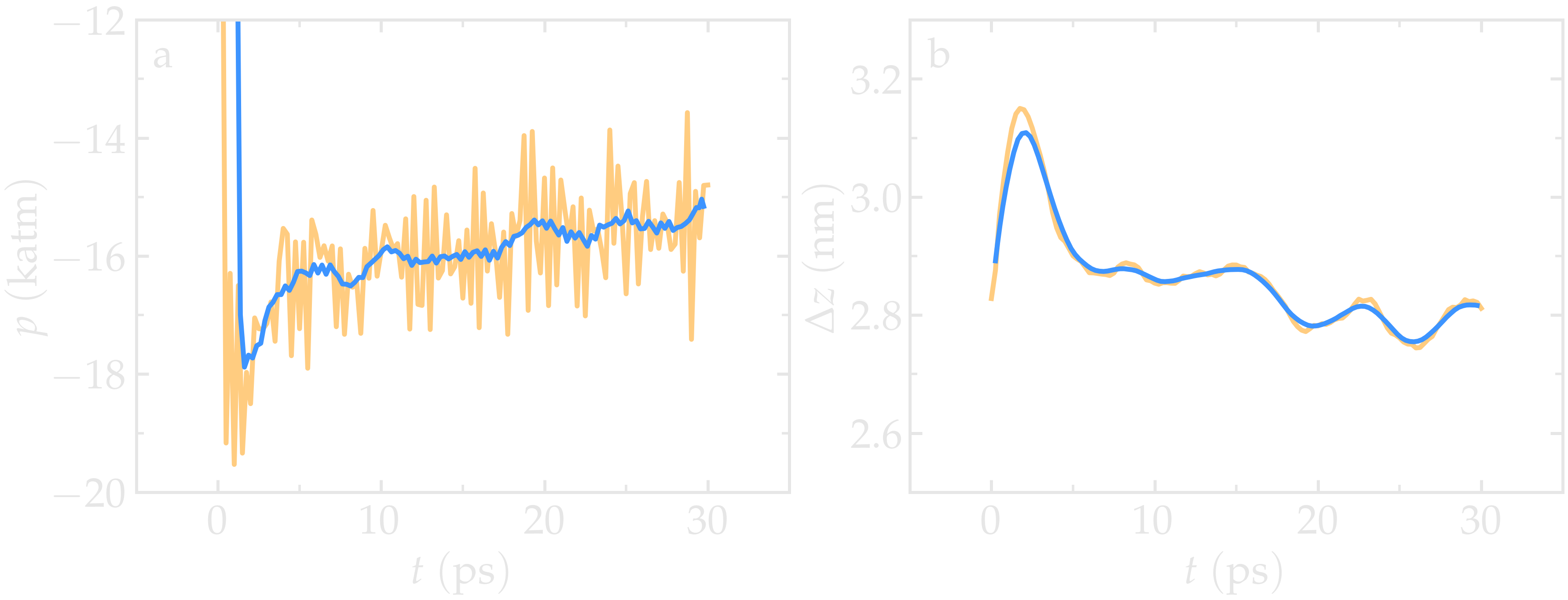
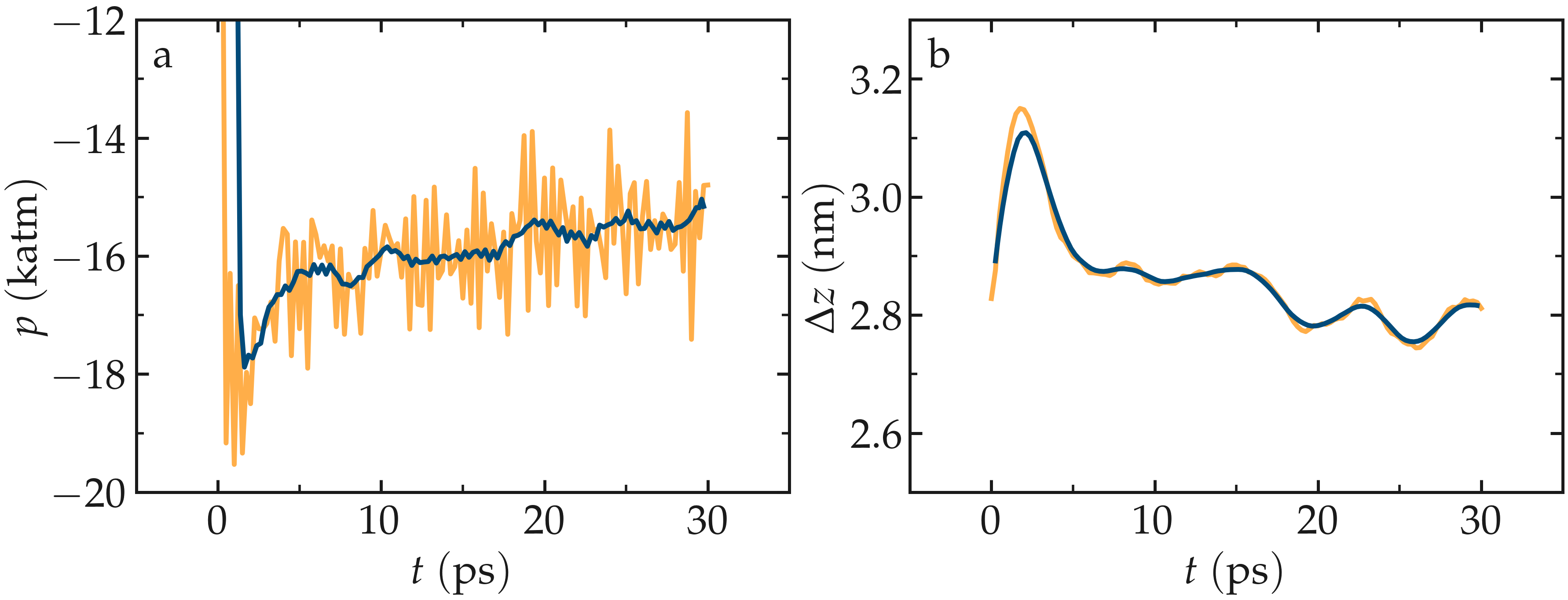
Figure: a) Pressure, \(p\), of the nanosheared electrolyte system as a function of the time, \(t\). b) Distance between the walls, \(\Delta z\), as a function of \(t\).

Imposed shearing

From the equilibrated configuration, let us impose a lateral motion on the two walls and shear the electrolyte.

If you are using LAMMPS-GUI

Open the last input file named shearing.lmp.

Create a new file, shearing.lmp, and copy the following into it:

boundary p p f
units real
atom_style full
bond_style harmonic
angle_style harmonic
pair_style lj/cut/tip4p/long O H O-H H-O-H 0.1546 12.0
kspace_style pppm/tip4p 1.0e-5
kspace_modify slab 3.0

read_data equilibrate.data

include parameters.inc
include groups.inc

To address the dynamics of the system, add the following lines to shearing.lmp:

compute Tfluid fluid temp/partial 0 1 1
fix mynvt1 fluid nvt temp 300 300 100
fix_modify mynvt1 temp Tfluid

compute Twall wall temp/partial 0 1 1
fix mynvt2 wall nvt temp 300 300 100
fix_modify mynvt2 temp Twall

fix myshk H2O shake 1.0e-5 200 0 b O-H a H-O-H
fix myrct all recenter NULL NULL 0
timestep 1.0

One key difference with the previous input is that, here, two thermostats are used, one for the fluid (mynvt1) and one for the solid (mynvt2). The combination of fix_modify with compute temp ensures that the correct temperature values are used by the thermostats. Using compute commands for the temperature with temp/partial 0 1 1 is intended to exclude the \(x\) coordinate from the thermalization, which is important since a large velocity will be imposed along the \(x\) direction.

Then, let us impose the velocity of the two walls by adding the following commands to shearing.lmp:

fix mysf1 walltop setforce 0 NULL NULL
fix mysf2 wallbot setforce 0 NULL NULL
velocity wallbot set -2e-4 NULL NULL
velocity walltop set 2e-4 NULL NULL

The setforce commands cancel the forces on walltop and wallbot. As a result, the atoms in these two groups will not experience any forces from the rest of the system. Consequently, in the absence of external forces, these atoms will conserve the initial velocities imposed by the two velocity commands.

Finally, let us generate images of the systems and print the values of the forces exerted by the fluid on the walls, as given by f_mysf1[1] and f_mysf2[1]. Add these lines to shearing.lmp:

dump mydmp all image 250 myimage-*.ppm type type shiny 0.1 box no 0.01 view 90 0 zoom 1.8
dump_modify mydmp backcolor white acolor O red adiam O 2 acolor H white adiam H 1 &
    acolor Na+ blue adiam Na+ 2.5 acolor Cl- cyan adiam Cl- 3 acolor WALL gray adiam WALL 3

thermo 250
thermo_modify temp Tfluid
thermo_style custom step temp etotal f_mysf1[1] f_mysf2[1]

Let us also extract the density and velocity profiles using the chunk/atom and ave/chunk commands. These commands are used to divide the system into bins and return the desired quantities, here the velocity along \(x\) (vx) within the bins. Add the following lines to shearing.lmp:

compute cc1 H2O chunk/atom bin/1d z 0.0 0.25
compute cc2 wall chunk/atom bin/1d z 0.0 0.25
compute cc3 ions chunk/atom bin/1d z 0.0 0.25

fix myac1 H2O ave/chunk 10 15000 200000 &
cc1 density/mass vx file shearing-water.dat
fix myac2 wall ave/chunk 10 15000 200000 &
cc2 density/mass vx file shearing-wall.dat
fix myac3 ions ave/chunk 10 15000 200000 &
cc3 density/mass vx file shearing-ions.dat

run 200000

Here, a bin size of \(0.25\,\text{Å}\) is used for the density profiles generated by the ave/chunk commands, and three .dat files are created for the water, the walls, and the ions, respectively. With values of 10 15000 200000, the velocity vx will be evaluated every 10 steps during the final 150,000 steps of the simulations. The result will be averaged and printed only once at the 200,000 th step.

Run the simulation using LAMMPS. The averaged velocity profile for the fluid is plotted below. As expected for such Couette flow geometry, the fluid velocity increases linearly along \(z\), and is equal to the walls velocities at the fluid-solid interfaces (no-slip boundary conditions).

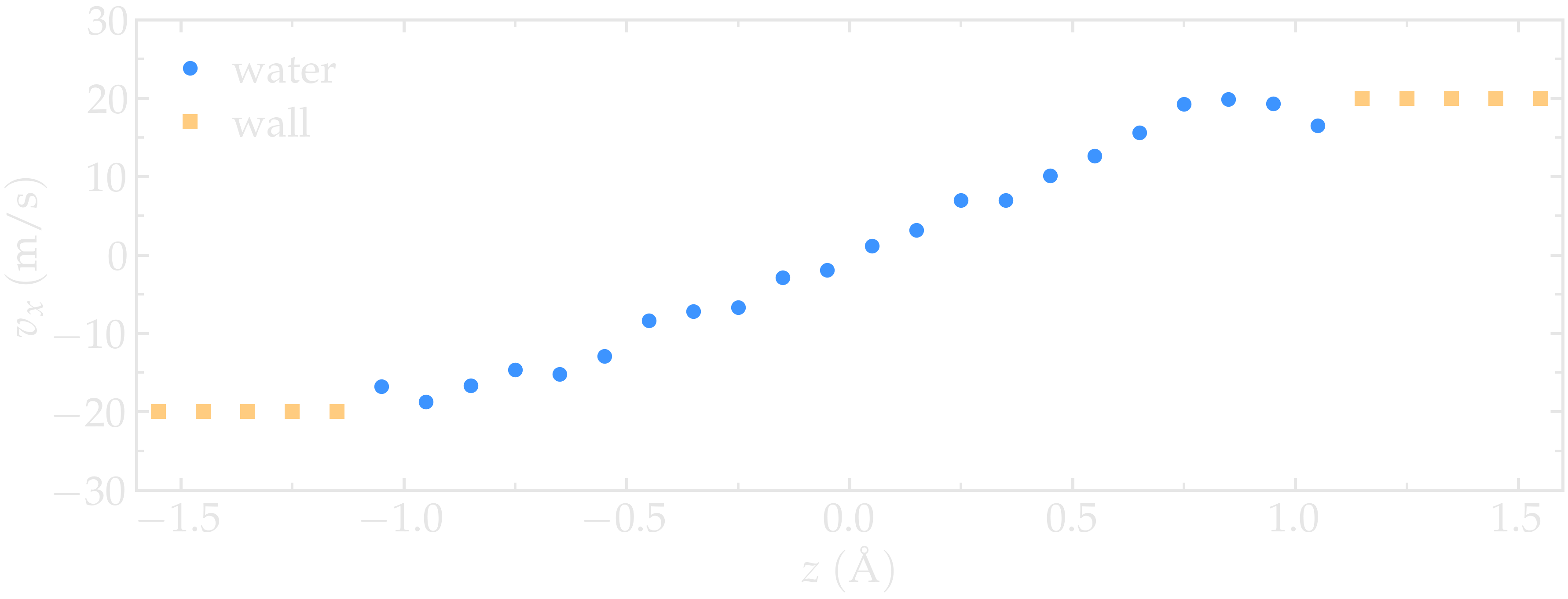
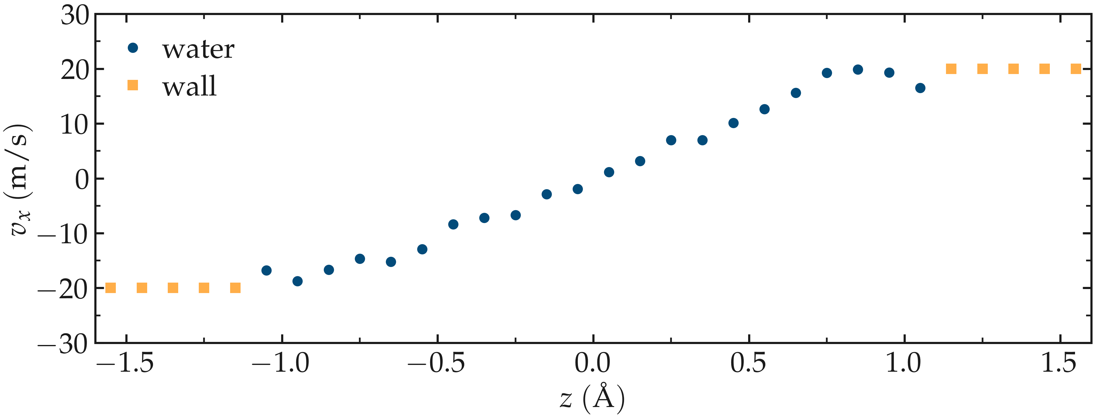
Figure: Velocity profiles for water (blue) and walls (orange) along the \(z\)-axis.

From the force applied by the fluid on the solid, one can extract the stress within the fluid, which enables the measurement of its viscosity \(\eta\) according to

(1)\[\eta = \tau / \dot{\gamma}\]

where \(\tau\) is the stress applied by the fluid on the shearing wall, and \(\dot{\gamma}\) the shear rate [37]. Here, the shear rate is approximately \(\dot{\gamma} = 20 \cdot 10^9\,\text{s}^{-1}\), the average force on each wall is given by f_mysf1[1] and f_mysf2[1] and is approximately \(2.7\,\mathrm{kcal/mol/Å}\) in magnitude. Using a surface area for the walls of \(A = 6 \cdot 10^{-18}\,\text{m}^2\), one obtains an estimate for the shear viscosity for the confined fluid of \(\eta = 3.1\,\text{mPa.s}\) using Eq. (1).

Note

The viscosity calculated at such a high shear rate may differ from the expected bulk value. In general, it is recommended to use a lower value for the shear rate. Note that for lower shear rates, the ratio of noise-to-signal is larger, and longer simulations are needed. Another important point to consider is that the viscosity of a fluid next to a solid surface is typically larger than in bulk due to interaction with the walls [38]. Therefore, one expects the present simulation to yield a viscosity that is slightly higher than what would be measured in the absence of walls.

Cite

You can access the input scripts and data files that are used in these tutorials from a dedicated Github repository. This repository also contains the full solutions to the exercises.

Going further with exercises

Induce a Poiseuille flow

Instead of inducing a shearing of the fluid using the walls, induce a net flux of the liquid in the direction tangential to the walls. The walls must be kept immobile.

Extract the velocity profile, and make sure that the resulting velocity profile is consistent with the Poiseuille equation, which can be derived from the Stokes equation \(\eta \nabla \textbf{v} = - \textbf{f} \rho\) where \(f\) is the applied force, \(\rho\) is the fluid density, \(\eta\) is the fluid viscosity.

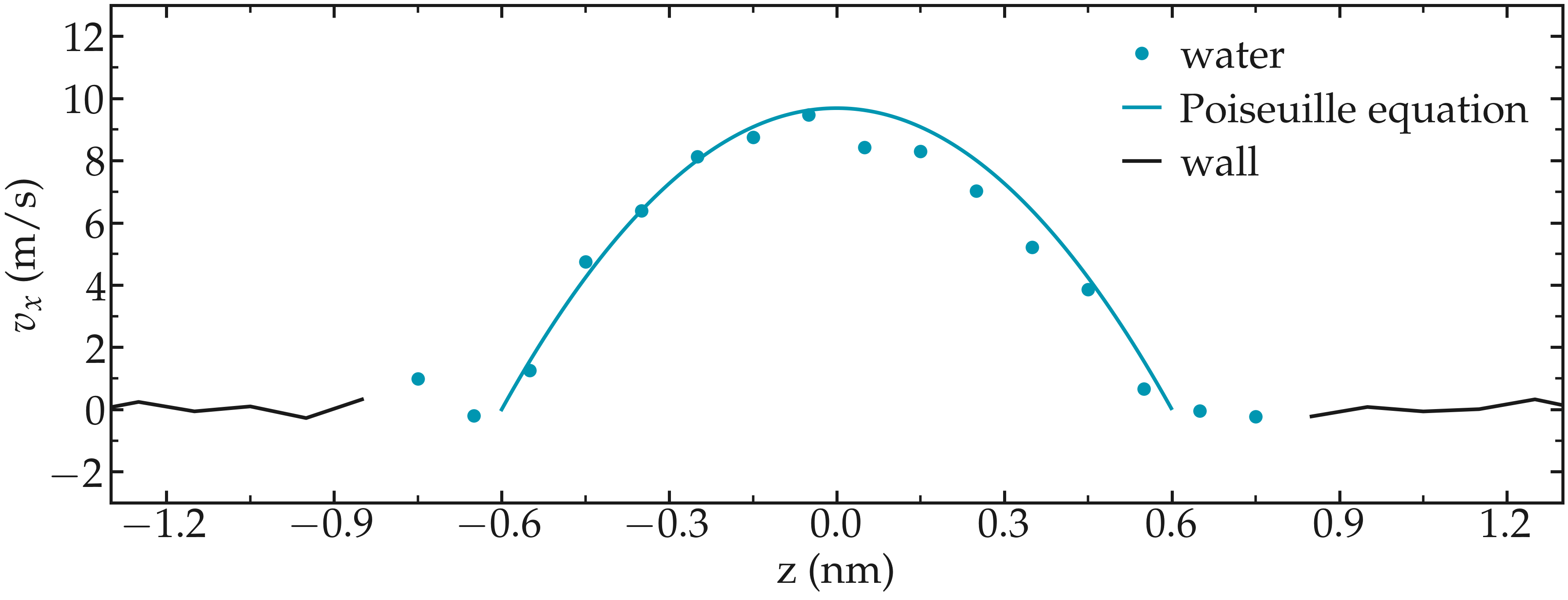
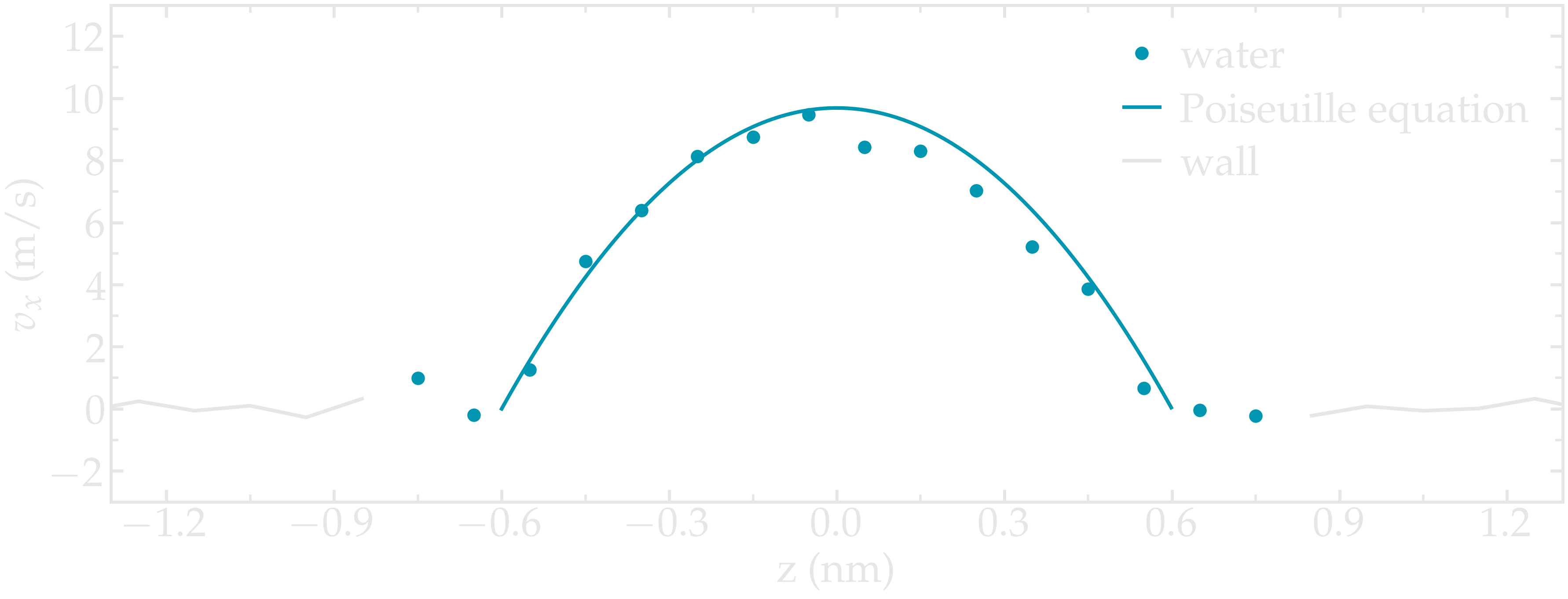
Figure: Velocity profiles of the water molecules along the z axis (disks). The line is the Poiseuille equation.

An important step is to choose the proper value for the additional force.