Reactive silicon dioxide
Simulating a chemically reactive structure
The objective of this tutorial is to demonstrate how the reactive force field ReaxFF can be used to calculate the partial charges of a system undergoing deformation, as well as the formation and breaking of chemical bonds [5, 40]. The system simulated in this tutorial is a block of silicon dioxide \(\text{SiO}_2\) which is deformed until it ruptures. Particular attention is given to the evolution of atomic charges during deformation, with a focus on tracking chemical reactions resulting from the deformation over time.
If you are completely new to LAMMPS, we recommend that you follow this tutorial on a simple Lennard-Jones fluid first.
Cite
If you find these tutorials useful, you can cite A Set of Tutorials for the LAMMPS Simulation Package [Article v1.0] by Simon Gravelle, Cecilia M. S. Alvares, Jacob R. Gissinger, and Axel Kohlmeyer, published in LiveCoMS, 6(1), 3037 (2025) [14].
This tutorial is compatible with the 22Jul2025 LAMMPS version.
Prepare and relax
The first step is to relax the structure with ReaxFF, which which will be achieved using molecular dynamics. To ensure the system equilibrates properly, we will monitor certain parameters over time, such as the system volume.
Create a folder if needed and place the initial input file, relax.lmp, into it. Then, open the file in a text editor of your choice, and copy the following into it:
units real
atom_style full

read_data silica.data
If you are using LAMMPS-GUI
To begin this tutorial, select Start Tutorial 5 from the
Tutorials menu of LAMMPS–GUI and follow the instructions.
The editor should display the following content corresponding to relax.lmp
So far, the input is very similar to what was seen in the previous tutorials.
Some basic parameters are defined (units and atom_style),
and a .data file is imported by the read_data command.
Looking for help with your project ?
Get guidance for your LAMMPS simulations and receive personalized advice for your project.
The initial topology given by silica.data
corresponds to a small amorphous silica structure. This structure was generated in a prior
simulation using the Vashishta force field [41].
If you open the silica.data
file, you will find in the Atoms section that all silicon atoms have a
charge of \(q = 1.1\,\text{e}\), and all oxygen atoms have a charge of \(q = -0.55\,\text{e}\).
Note
Assigning the same charge to all atoms of the same type is common with many force fields, including the force fields used in the previous tutorials. This changes once ReaxFF is used: the charge of each atom will adjust to its local environment through charge equilibration.
Next, copy the following three crucial lines into the relax.lmp file:
pair_style reaxff NULL safezone 3.0 mincap 150
pair_coeff * * ffield.reax.CHOFe Si O
fix myqeq all qeq/reaxff 1 0.0 10.0 1.0e-6 reaxff maxiter 400
In this case, the pair_style reaxff is used without a control file (see note below). The
safezone and mincap keywords are added to prevent
allocation issues, which sometimes can trigger segmentation faults and
bondchk errors. The pair_coeff command uses the ffield.reax.CHOFe
file, which should have been downloaded during the tutorial set up. Finally, the
fix qeq/reaxff is used to perform charge equilibration [42],
which occurs at every step. The values 0.0 and 10.0 represent the
low and the high cutoffs, respectively, and \(1.0 \text{e} -6\) is the tolerance,
i.e., the precision to which the atomic charges are equilibrated during the
charge equilibration process.
Note
The pair_style reaxff command optionally accepts a control file,
which defines control variables such as
global parameters of the ReaxFF potential, as well as performance and output settings.
If no control file is provided, as in this tutorial, LAMMPS uses its default values,
which correspond to those in Adri van Duin’s original stand-alone ReaxFF code [5].
The maxiter sets an upper limit to the number of attempts to
equilibrate the charge.
Next, add the following commands to the relax.lmp file to track the evolution of the charges during the simulation:
group grpSi type Si
group grpO type O
variable qSi equal charge(grpSi)/count(grpSi)
variable qO equal charge(grpO)/count(grpO)
variable vq atom q
The definition of the equal style variables qSi and qO make
use of functions pre-defined within LAMMPS that allow
calculating the total charge of atoms belonging to a group
(charge()) and the total number of atoms in the group
(count()). To print the averaged charges qSi and qO using the
thermo_style command, and create images of the system. Add the
following lines to relax.lmp:
thermo 100
thermo_style custom step temp etotal press vol v_qSi v_qO
dump viz all image 100 myimage-*.ppm q type shiny 0.1 box no 0.01 view 180 90 zoom 2.3 size 1200 500
dump_modify viz adiam Si 2.6 adiam O 2.3 backcolor white amap -1 2 ca 0.0 3 min royalblue 0 green max orangered
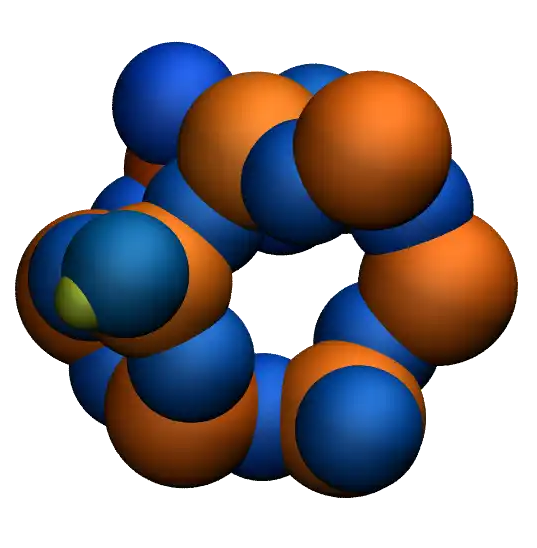
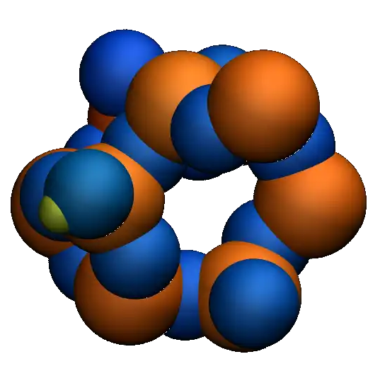
Here, the atoms are colored by their charges q, ranging from royal blue
(when \(q=-1\,\text{e}\)) to orange-red (when \(q=2\,\text{e}\)).
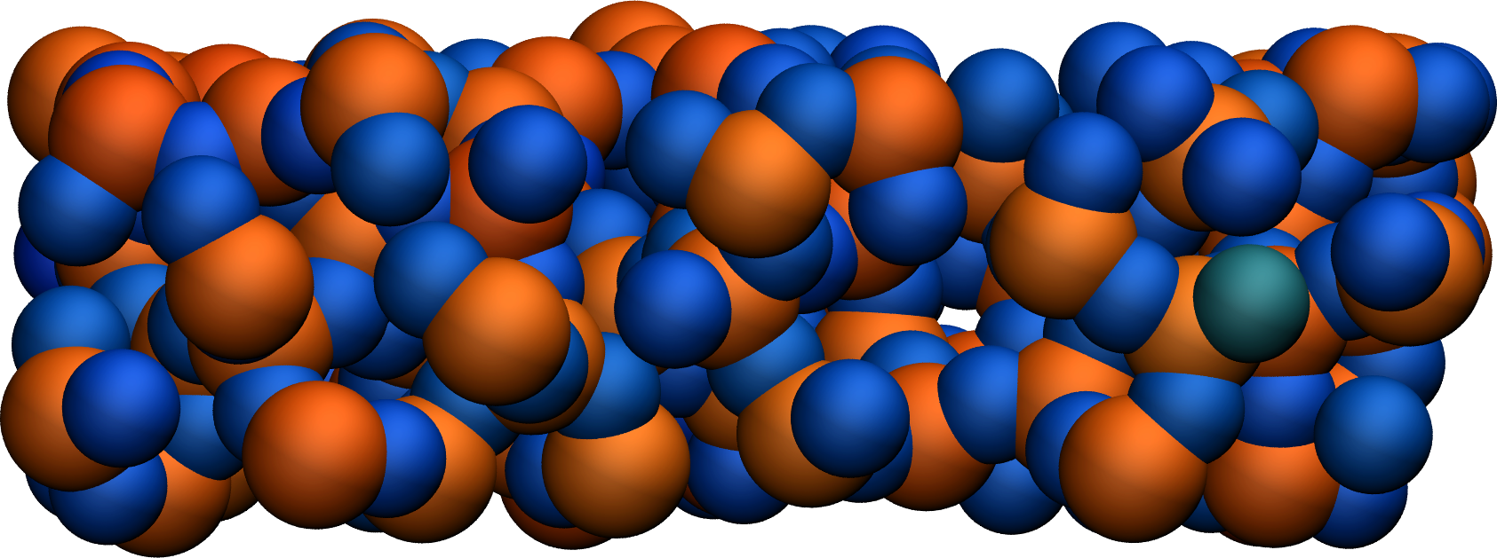
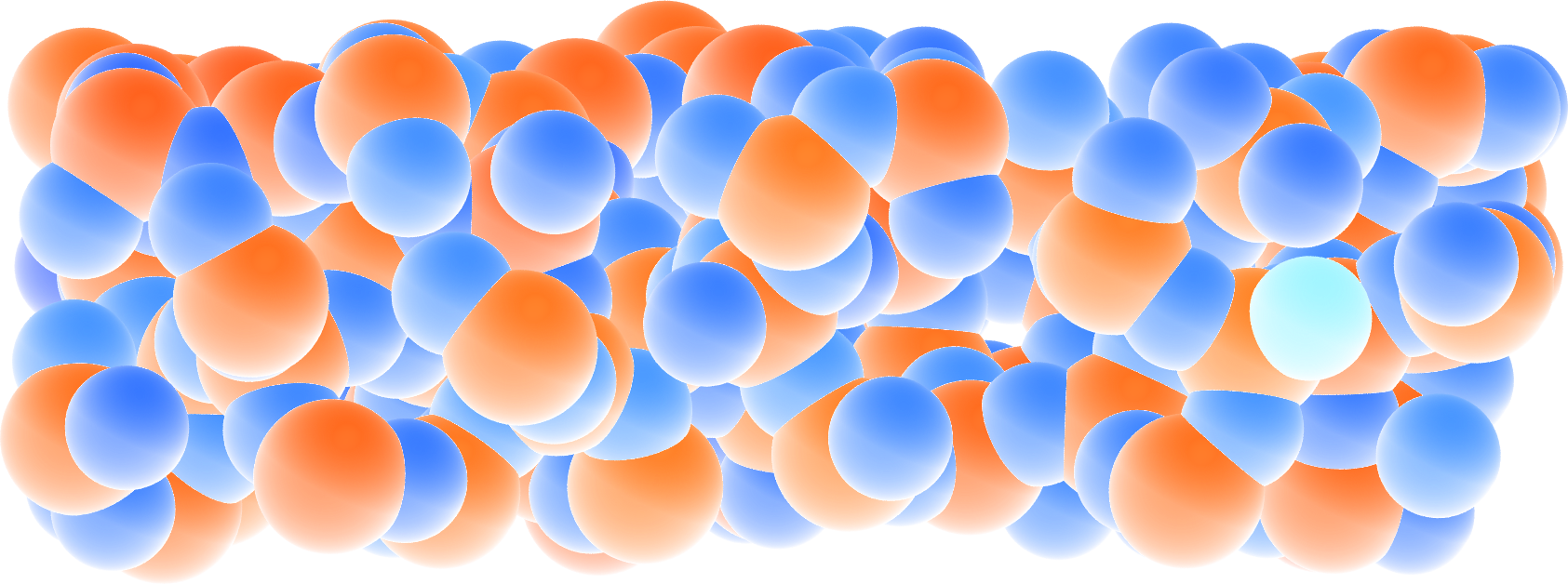
Figure: Amorphous silicon oxide. The atoms are colored by their charges. Dangling oxygen groups appear in greenish, bulk Si atoms with a charge of about \(1.8~\text{e}\) appear in red/orange, and bulk O atoms with a charge of about \(-0.9 ~ \text{e}\) appear in blue.
We can generate histograms of the charges for each atom type using
fix ave/histo commands:
fix myhis1 grpSi ave/histo 10 500 5000 -1.5 2.5 1000 v_vq file relax-Si.histo mode vector
fix myhis2 grpO ave/histo 10 500 5000 -1.5 2.5 1000 v_vq file relax-O.histo mode vector
The fix ave/histo command samples values
over a group of atoms and builds a histogram over a specified range divided into
bins. In this tutorial, it is used to monitor the charge distributions
of silicon and oxygen atoms. The parameters 10 500 5000 specify how often
the histogram is updated and averaged, -1.5 2.5 set the value range,
1000 is the number of bins, and v\_vq is the variable being histogrammed.
We can also use the fix reaxff/species to evaluate what species are
present within the simulation. It will be useful later when the system is deformed,
and bonds are broken:
fix myspec all reaxff/species 5 1 5 relax.species element Si O
Here, the information will be printed every 5 steps in a file called relax.species. Let us perform a very short run using the anisotropic NPT command and relax the density of the system:
velocity all create 300.0 32028
fix mynpt all npt temp 300.0 300.0 100 aniso 1.0 1.0 1000
timestep 0.5

run 5000

write_data relax.data nofix
Note
With the aniso keyword, the three dimensions of the simulation box can change independently. This is particularly relevant for solids and other systems where anisotropic stresses may develop.
The write_data command is used with the nofix keyword to print a data file
without extra sections from the reaxff/species command.
Run the relax.lmp file using LAMMPS. As seen from relax.species,
only one species is detected, called O384Si192, representing the entire system.
As the simulation progresses, the charge of every atom fluctuates because it is adjusting to the local environment of the atom. It is also observed that the averaged charges for silicon and oxygen atoms fluctuate significantly at the beginning of the simulation, corresponding to a rapid change in the system volume, which causes interatomic distances to shift quickly. The atoms with the most extreme charges are located at structural defects, such as dangling oxygen groups.
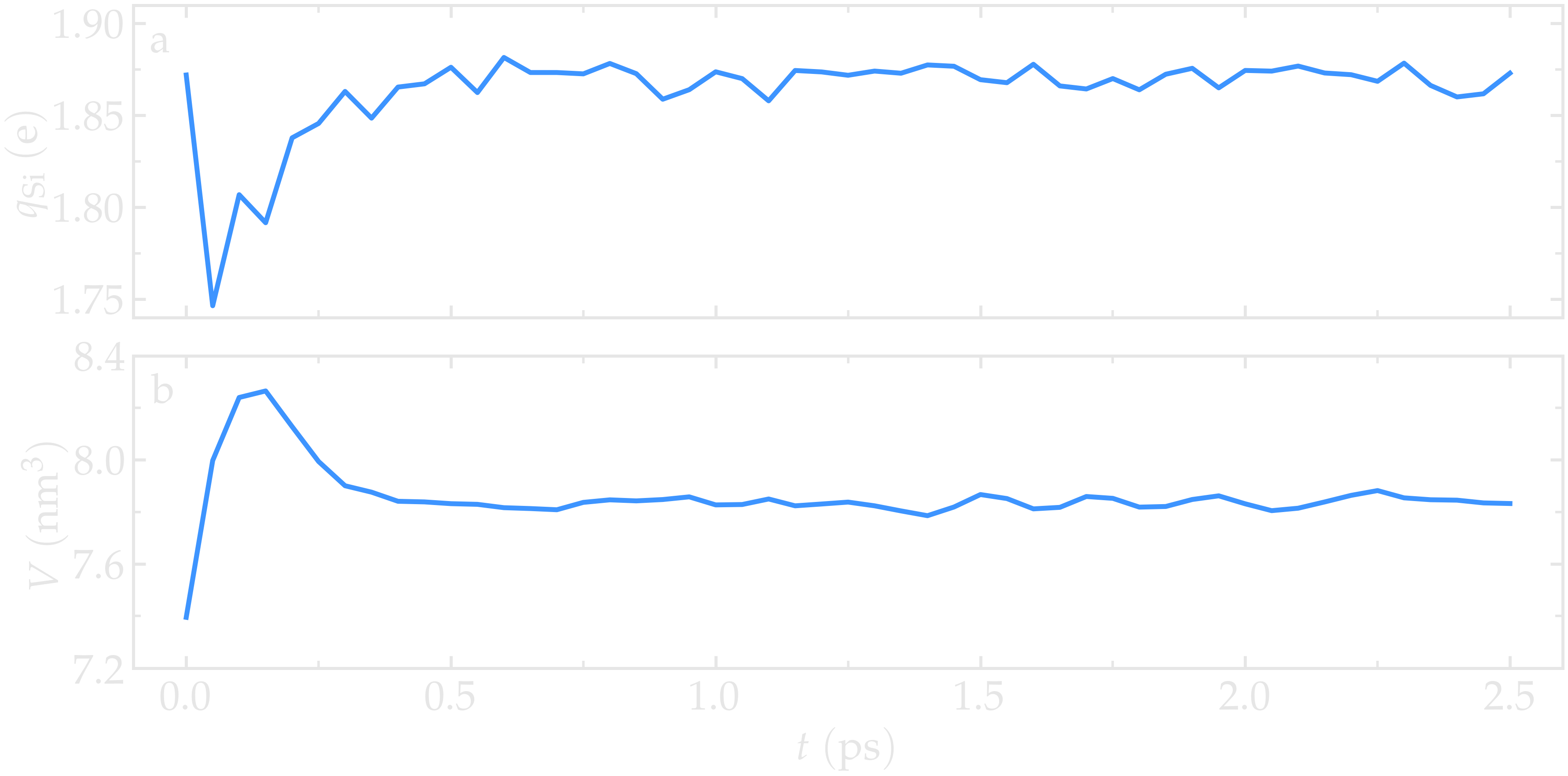
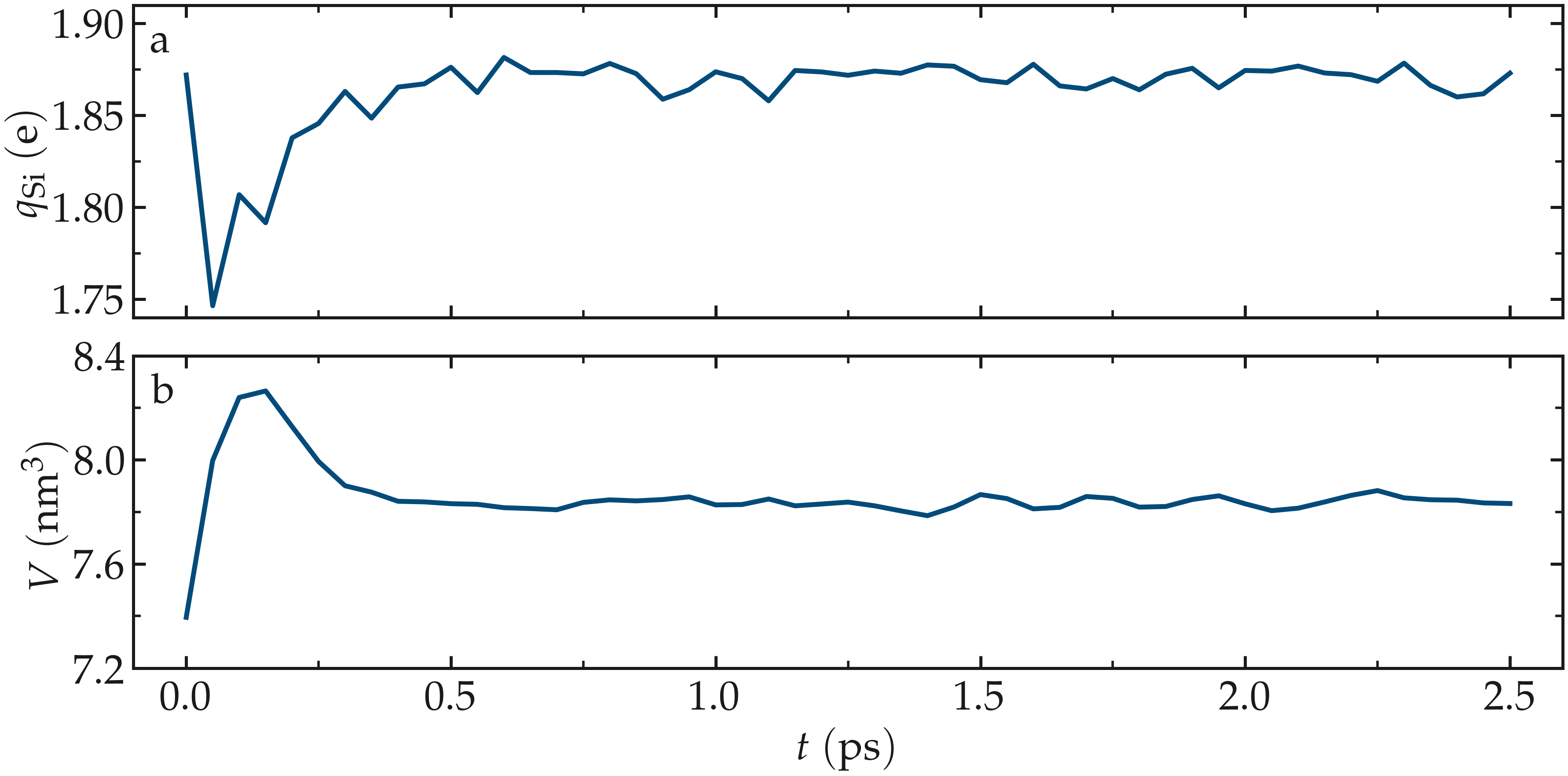
Figure: a) Average charge per atom of the silicon, \(q_\text{Si}\), atoms as a function of time, \(t\), during equilibration of the \(\text{SiO}_2\) system. b) Volume of the system, \(V\), as a function of \(t\).
Figure: A slice of the amorphous silica, where atoms are colored by their charges. Dangling oxygen groups appear in greenish, bulk Si atoms with a charge of about \(1.8~\text{e}\) appear in red/orange, and bulk O atoms with a charge of about \(-0.9~\text{e}\) appear in blue.
Finally, the generated .histo files can be used to plot the probability distributions, \(P(q)\).
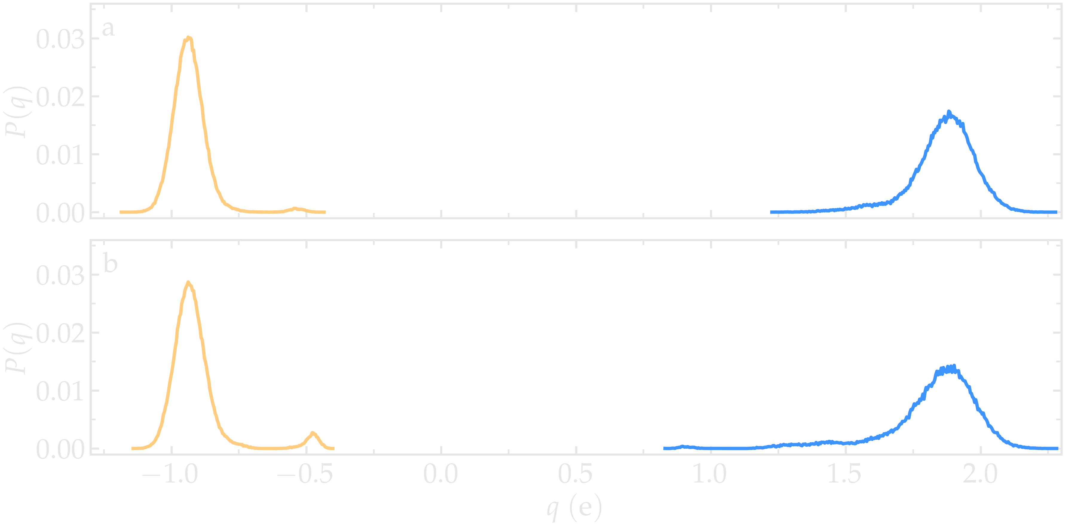
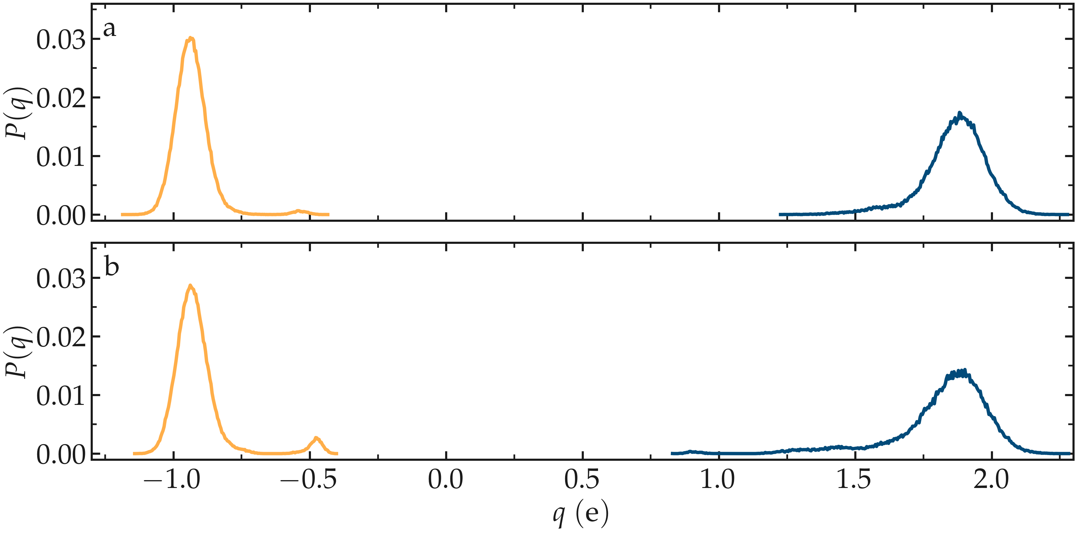
Figure: a) Probability distributions of charge of silicon (positive, blue) and oxygen (negative, orange) atoms during the equilibration of the \(\text{SiO}_2\) system. b) Same probability distributions as in panel (a) after the deformation.
Deform the structure
Let us apply a deformation to the structure to force some \(\text{Si}-\text{O}\) bonds to break (and eventually re-assemble). Open the deform.lmp file, which must contain the following lines:
units real
atom_style full

read_data relax.data

pair_style reaxff NULL safezone 3.0 mincap 150
pair_coeff * * ffield.reax.CHOFe Si O
fix myqeq all qeq/reaxff 1 0.0 10.0 1.0e-6 reaxff maxiter 400

group grpSi type Si
group grpO type O
variable qSi equal charge(grpSi)/count(grpSi)
variable qO equal charge(grpO)/count(grpO)
variable vq atom q

thermo 200
thermo_style custom step temp etotal press vol v_qSi v_qO
dump viz all image 100 myimage-*.ppm q type shiny 0.1 box no 0.01 view 180 90 zoom 2.3 size 1200 500
dump_modify viz adiam Si 2.6 adiam O 2.3 backcolor white amap -1 2 ca 0.0 3 min royalblue 0 green max orangered

fix myhis1 grpSi ave/histo 10 500 5000 -1.5 2.5 1000 v_vq file deform-Si.histo mode vector
fix myhis2 grpO ave/histo 10 500 5000 -1.5 2.5 1000 v_vq file deform-O.histo mode vector
fix myspec all reaxff/species 5 1 5 deform.species element Si O
The only difference with the previous relax.lmp file is the path to the relax.data file.
Next, let us use fix nvt instead of fix npt to apply a
Nosé-Hoover thermostat without a barostat:
fix mynvt all nvt temp 300.0 300.0 100
timestep 0.5
Here, no barostat is used because the change in the box volume will be imposed
by the fix deform, see below.
Let us run for 5000 steps without deformation, then apply the fix deform
to progressively elongate the box along the \(x\)-axis during 25000 steps. Add
the following line to deform.lmp:
run 5000

fix mydef all deform 1 x erate 5e-5

run 25000

write_data deform.data nofix
The fix deform command applies a continuous deformation
by elongating the simulation box along the x-axis at a constant engineering
shear strain rate, specified by erate, of \(5 \times 10^{-5}~\text{fs}^{-1}\).
Run the deform.lmp file using LAMMPS. During the deformation, the charge values progressively evolve until the structure eventually breaks down. After the structure breaks down, the charges equilibrate near new average values that differ from the initial averages. The difference between the initial and the final charges can be explained by the presence of defects, as well as new solid/vacuum interfaces, and the fact that surface atoms typically have different charges compared to bulk atoms. You can also see a sharp increase in temperature during the rupture of the material.
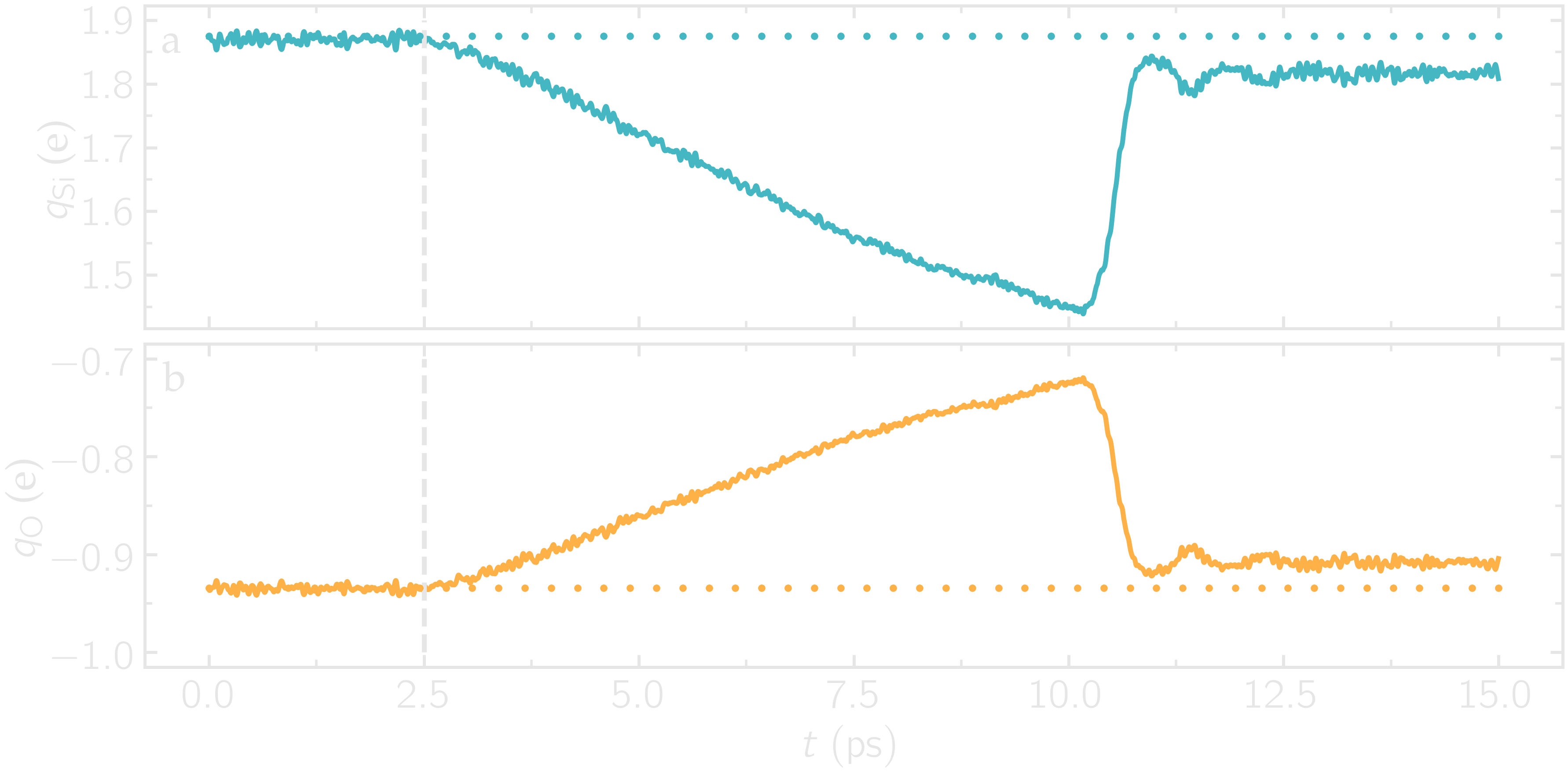
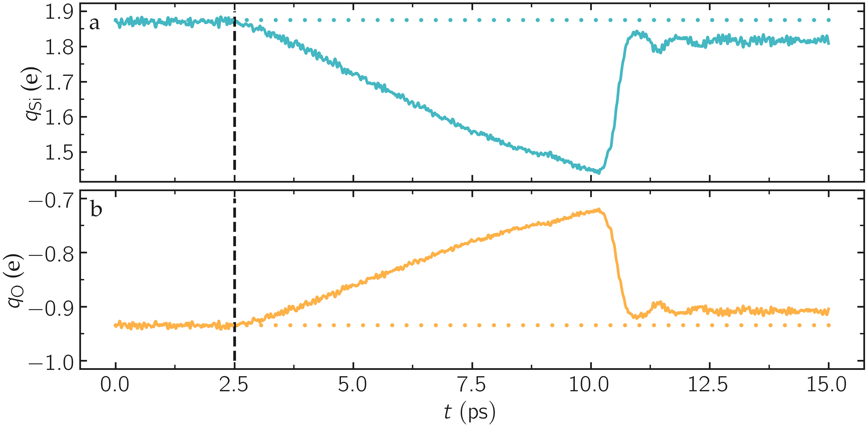
Figure: a) Average charge per atom of the silicon, \(q_\text{Si}\), atoms as a function of time, \(t\), during deformation of the \(\text{SiO}_2\) system. The break down of the silica structure occurs near \(t = 11\) ps. b) Temperature, \(T\), of the system as a function of \(t\).
You can examine the charge distribution after deformation, as well as during deformation. As expected, the final charge distribution slightly differs from the previously calculated one. If no new species were formed during the simulation, the deform.species file should look like this:
#  Timestep   No_Moles   No_Specs  O384Si192
        5            1          1          1
(...)
#  Timestep   No_Moles   No_Specs  O384Si192
    30000            1          1          1
Sometimes, \(\text{O}_2\) molecules are formed during the deformation. If this occurs,
a new column O2 appears in the deform.species file.
Decorate the surface
Under ambient conditions, some of the surface \(\text{SiO}_2\) atoms become chemically passivated by forming covalent bonds with hydrogen (H) atoms [43]. We will add hydrogen atoms randomly to the cracked silica and observe how the system evolves. To do so, we first need to modify the previously generated data file deform.data and make space for a third atom type. Copy deform.data, name the copy deform-mod.data, and modify the first lines of deform-mod.data as follows:
576 atoms
3 atom types

(...)

Atom Type Labels

1 Si
2 O
3 H

Masses

Si 28.0855
O 15.999
H 1.008

(...)
Open the decorate.lmp file, which must contain the following lines:
units real
atom_style full

read_data deform-mod.data
displace_atoms all move -12 0 0 # optional

pair_style reaxff NULL safezone 3.0 mincap 150
pair_coeff * * ffield.reax.CHOFe Si O H
fix myqeq all qeq/reaxff 1 0.0 10.0 1.0e-6 reaxff maxiter 400
The displace_atoms command is used to move the center of the
crack near the center of the box. This step is optional but makes for a nicer
visualization. A different value for the shift may be needed in
your case, depending on the location of the crack. A difference with the previous
input is that three atom types are specified in the pair_coeff command, i.e.
Si O H.
Then, let us adapt some familiar commands to measure the charges of all three types of atoms, and output the charge values into log files:
group grpSi type Si
group grpO type O
group grpH type H
variable qSi equal charge(grpSi)/count(grpSi)
variable qO equal charge(grpO)/count(grpO)
variable qH equal charge(grpH)/(count(grpH)+1e-10)

thermo 5
thermo_style custom step temp etotal press v_qSi v_qO v_qH

dump viz all image 100 myimage-*.ppm q type shiny 0.1 box no 0.01 view 180 90 zoom 2.3 size 1200 500
dump_modify viz adiam Si 2.6 adiam O 2.3 adiam H 1.0 backcolor white amap -1 2 ca 0.0 3 min royalblue 0 green max orangered

fix myspec all reaxff/species 5 1 5 decorate.species element Si O H
The commands above are, once again, similar to the ones of the previous script.
Here, the \(+1 \mathrm{e}{-10}\) was added to the denominator of the variable qH
to avoid dividing by 0 at the beginning of the simulation, as no hydrogen atoms exists in
the simulation domain yet. Finally, let us create a loop with 10 steps, and
create two hydrogen atoms at random locations at every step:
fix mynvt all nvt temp 300.0 300.0 100
timestep 0.5

label loop
variable a loop 10

variable seed equal 35672+${a}
create_atoms 3 random 2 ${seed} NULL overlap 2.6 maxtry 50

run 2000

next a
jump SELF loop
Run the simulation with LAMMPS. When the simulation is over, it can be seen from the decorate.species file that all the created hydrogen atoms reacted with the \(\text{SiO}_{2}\) structure to form surface groups (such as hydroxyl (-OH) groups).
(...)
# Timestep   No_Moles No_Specs H20O384Si192
20000      1        1        1
At the end of the simulation, hydroxyl (-OH) groups can be seen at the interfaces.
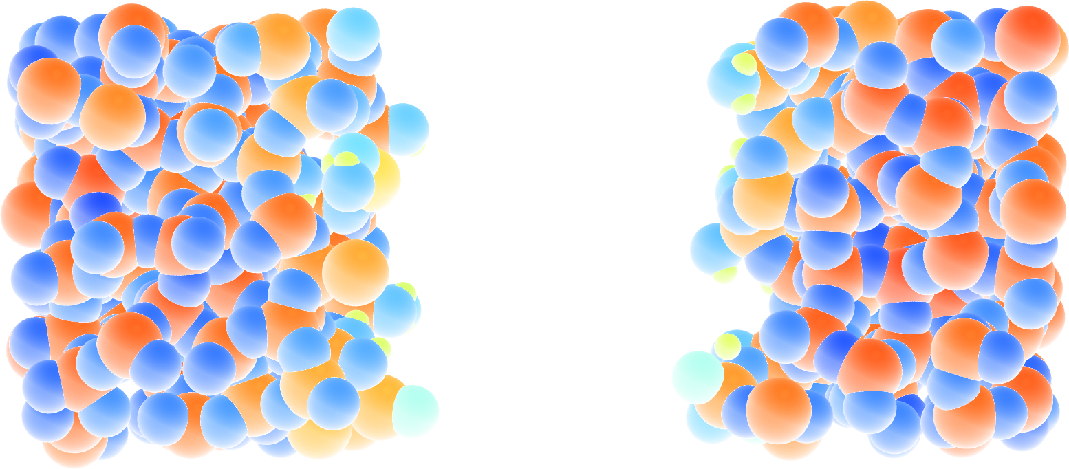
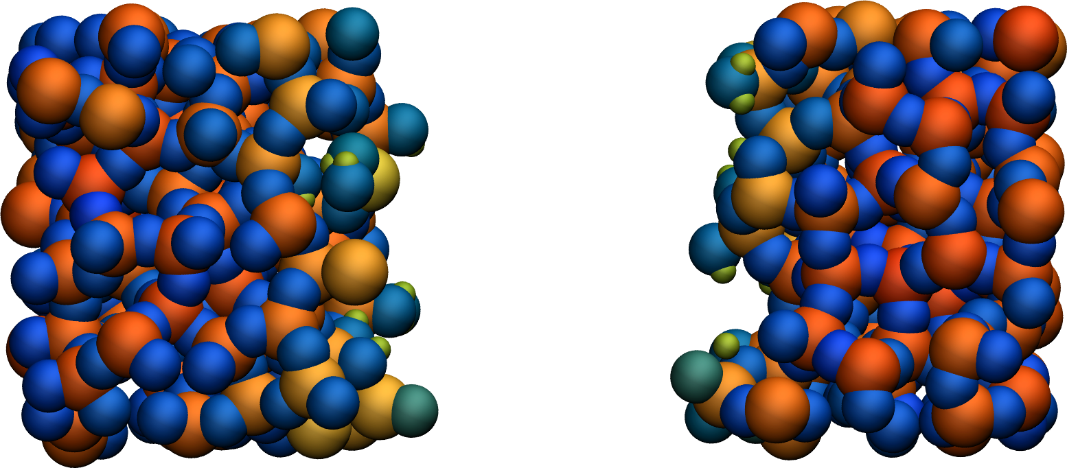
Figure: Cracked silicon oxide after the addition of hydrogen atoms. The atoms are colored by their charges, with the newly added hydrogen atoms appearing as small greenish spheres.
Cite
You can access the input scripts and data files that are used in these tutorials from a dedicated GitHub repository. This repository also contains the full solutions to the exercises.
Going further with exercises
Hydrate the structure
Add water molecules to the current structure, and follow the reactions over time.
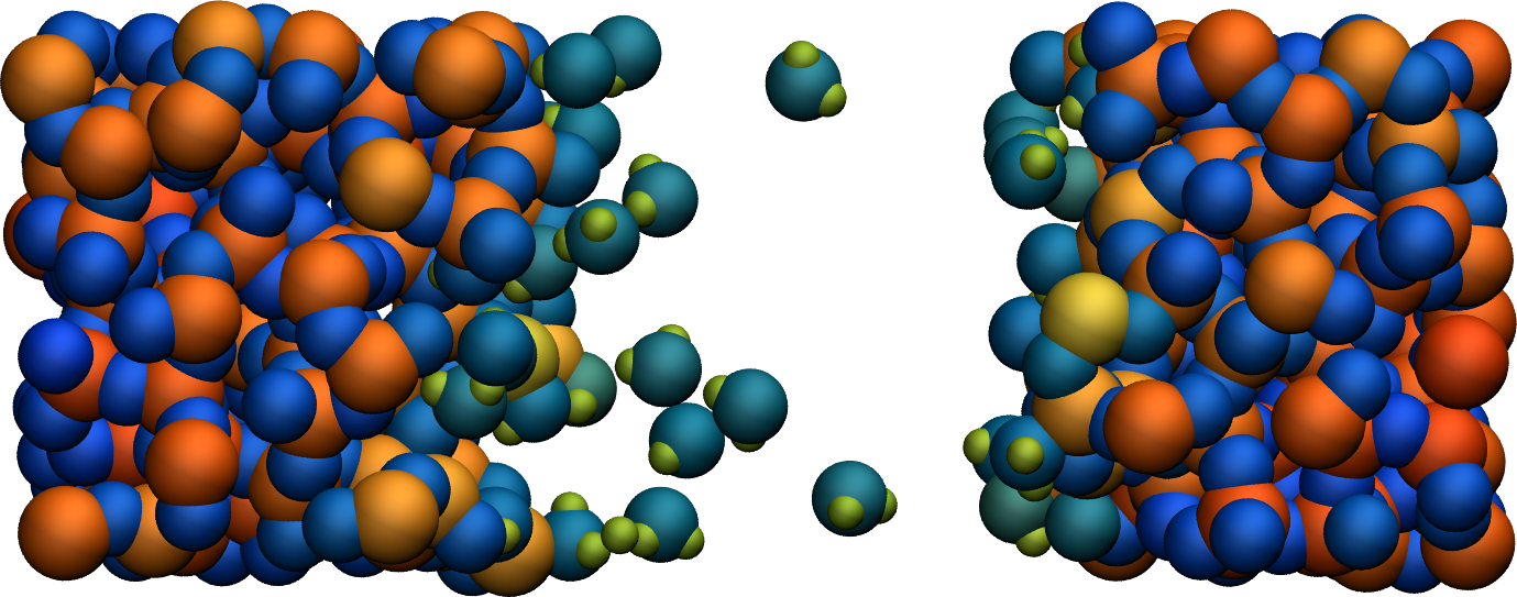
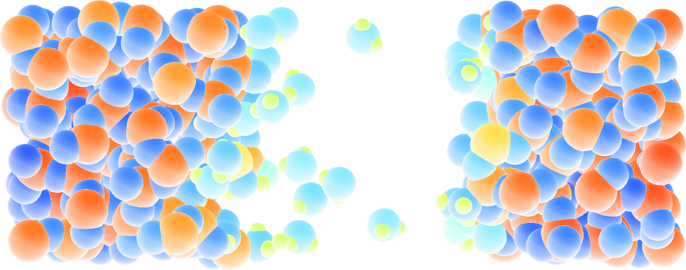
Figure: Cracked silicon oxide after the addition of water molecules. The atoms are colored by their charges.
A slightly acidic bulk solution
Create a bulk water system with a few hydronium ions (\(H_3O^+\) or \(H^+\)) using ReaxFF. The addition of hydronium ions will make the system acidic.
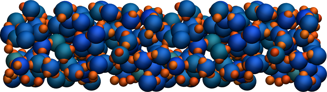
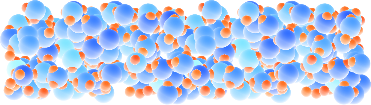
Figure: Slightly acidic bulk water simulated with ReaxFF. The atoms are colored by their charges.