Water adsorption in silica

Dealing with a varying number of molecules

The objective of this tutorial is to combine molecular dynamics and grand canonical Monte Carlo simulations to compute the adsorption of water molecules in cracked silica material. This tutorial illustrates the use of the grand canonical ensemble in molecular simulation, an open ensemble where the number of atoms or molecules in the simulation box can vary. By employing the grand canonical ensemble, we will set the chemical potential of water within a nanoporous \(\text{SiO}_2\) structure.

If you are completely new to LAMMPS, we recommend that you follow this tutorial on a simple Lennard-Jones fluid first.

Cite

If you find these tutorials useful, you can cite A Set of Tutorials for the LAMMPS Simulation Package by Simon Gravelle, Jacob R. Gissinger, and Axel Kohlmeyer (2025) [14]. You can access the full paper on arXiv.

This tutorial is compatible with the 29Aug2024 (update 2) LAMMPS version.

Generation of the silica block

To begin this tutorial, if you are using LAMMPS–GUI, select Start Tutorial 6 from the Tutorials menu and follow the instructions. Alternatively, if you are not using LAMMPS–GUI, create a new folder and add a file named generate.lmp. Open the file in a text editor and paste in the following content:

units metal
boundary p p p
atom_style full
pair_style vashishta
neighbor 1.0 bin
neigh_modify delay 1

The main difference from some of the previous tutorials is the use of the Vashishta pair style. The Vashishta potential implicitly models atomic bonds through energy terms dependent on interatomic distances and angles [40].

Let us create a box for two atom types, Si of mass 28.0855 g/mol and O of mass 15.9994 g/mol. Add the following lines to generate.lmp:

region box block -18.0 18.0 -9.0 9.0 -9.0 9.0
create_box 2 box
labelmap atom 1 Si 2 O
mass Si 28.0855
mass O 15.9994
create_atoms Si random 240 5802 box overlap 2.0 maxtry 500
create_atoms O random 480 1072 box overlap 2.0 maxtry 500

The create_atoms commands are used to place 240 Si atoms, and 480 atoms, respectively. This corresponds to an initial density of approximately \(2 \, \text{g/cm}^3\), which is close to the expected final density of amorphous silica at 300 K.

Now, specify the pair coefficients by indicating that the first atom type is Si and the second is O:

pair_coeff * * SiO.1990.vashishta Si O

Ensure that the SiO.1990.vashishta file is located in the same directory as generate.lmp.

Next, add a dump image command to generate.lmp to follow the evolution of the system with time:

dump viz all image 250 myimage-*.ppm type type shiny 0.1 box no 0.01 view 180 90 zoom 3.4 size 1700 700
dump_modify viz backcolor white acolor Si yellow adiam Si 2.5 acolor O red adiam O 2

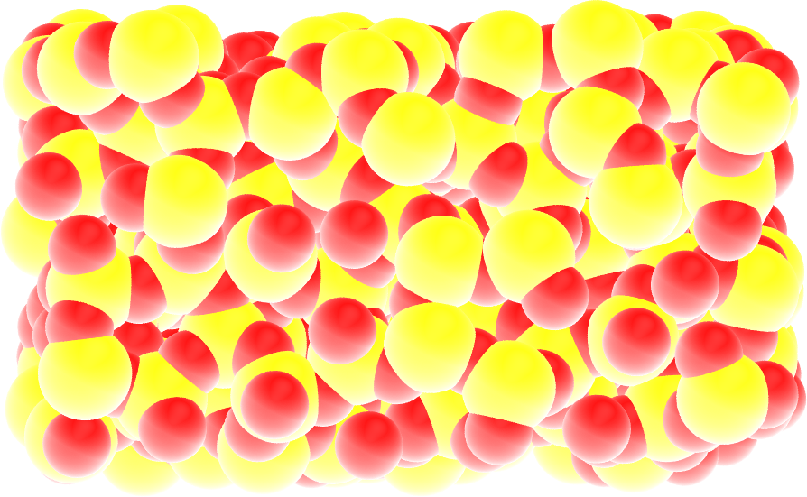
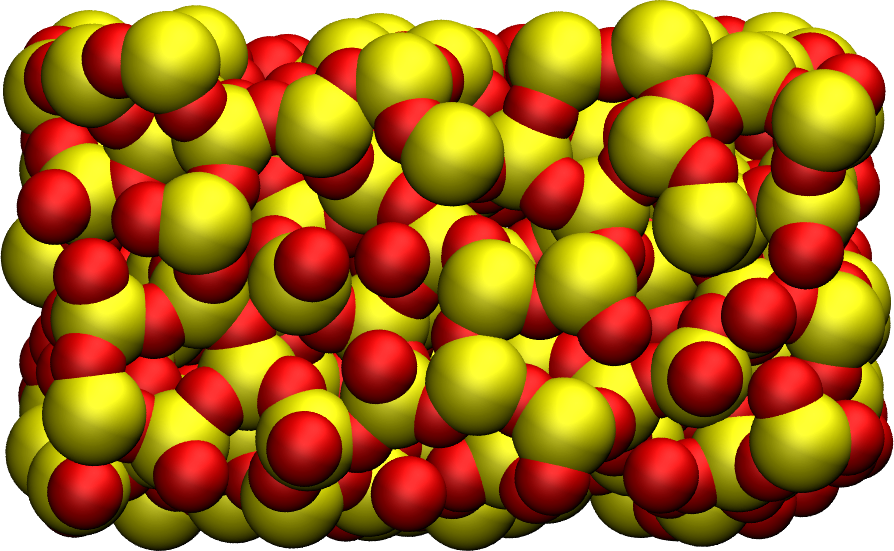
Figure: Amorphous silica (\(\text{SiO}_2\)). Silicon atoms are represented in yellow, and oxygen atoms in red.

Let us also print the box volume and system density, alongside the temperature and total energy:

thermo 250
thermo_style custom step temp etotal vol density

Finally, let us implement the annealing procedure which consists of three consecutive runs. This procedure was inspired by Ref. [43]. First, to melt the system, a \(10\,\text{ps}\) phase at \(T = 6000\,\text{K}\) is performed:

velocity all create 6000 8289 rot yes dist gaussian
fix mynvt all nvt temp 6000 6000 0.1
timestep 0.001
run 10000

Next, a second phase, during which the system is cooled down from \(T = 6000\,\text{K}\) to \(T = 300\,\text{K}\), is implemented as follows:

fix mynvt all nvt temp 6000 300 0.1
run 30000

In the third step, the system is equilibrated at the final desired conditions, \(T = 300\,\text{K}\) and \(p = 1\,\text{atm}\), using an anisotropic pressure coupling:

unfix mynvt

fix mynpt all npt temp 300 300 0.1 aniso 1 1 1
run 10000

write_data generate.data

Here, an anisotropic barostat is used. Anisotropic barostats adjust the dimensions independently, which is generally suitable for a solid phase.

Run the simulation using LAMMPS. From the Charts window, the temperature evolution can be observed, showing that it closely follows the desired annealing procedure. The evolution of the box dimensions over time confirms that the box deformed during the last stage of the simulation. After the simulation completes, the final LAMMPS topology file called generate.data will be located next to generate.lmp.

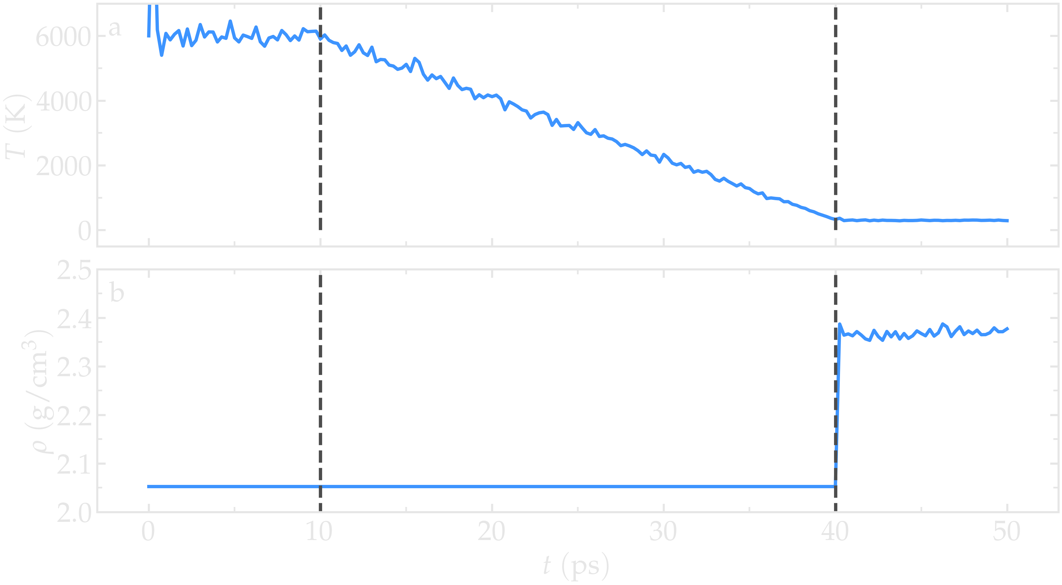
Figure: a) Temperature, \(T\), as a function of time, \(t\), during the annealing of the silica system. b) System density, \(\rho\), during the annealing process. The vertical dashed lines mark the transition between the different phases of the simulation.

Cracking the silica

Create a new file called cracking.lmp, and copy the following familiar lines:

units metal
boundary p p p
atom_style full
pair_style vashishta
neighbor 1.0 bin
neigh_modify delay 1

read_data generate.data

pair_coeff * * SiO.1990.vashishta Si O

dump viz all image 250 myimage-*.ppm type type shiny 0.1 box no 0.01 view 180 90 zoom 3.4 size 1700 700
dump_modify viz backcolor white acolor Si yellow adiam Si 2.5 acolor O red adiam O 2

thermo 250
thermo_style custom step temp etotal vol density

If you are using LAMMPS-GUI

Open the cracking.lmp file.

Let us progressively increase the size of the box in the \(x\) direction, forcing the silica to deform and eventually crack. To achive this, the fix deform command is used, with a rate of \(0.005\,\text{ps}^{-1}\). Add the following lines to the cracking.lmp file:

timestep 0.001
fix nvt1 all nvt temp 300 300 0.1
fix mydef all deform 1 x erate 0.005
run 50000

write_data cracking.data

The fix nvt command is employed to control the temperature of the system. As observed from the generated images, the atoms progressively adjust to the changing box dimensions. At some point, bonds begin to break, leading to the appearance of dislocations.

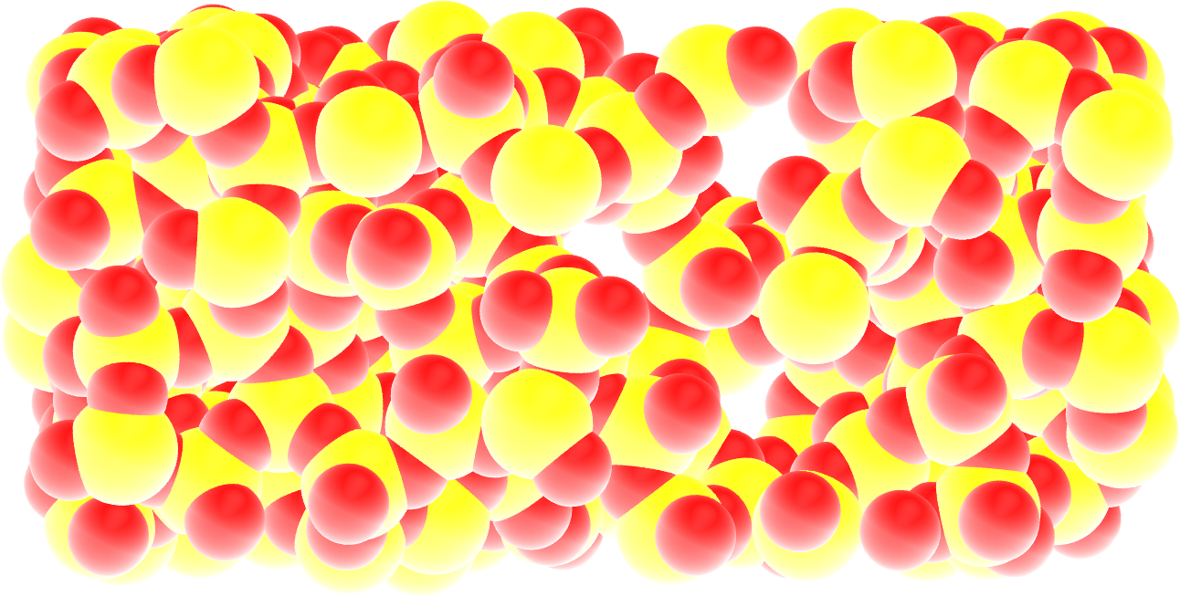
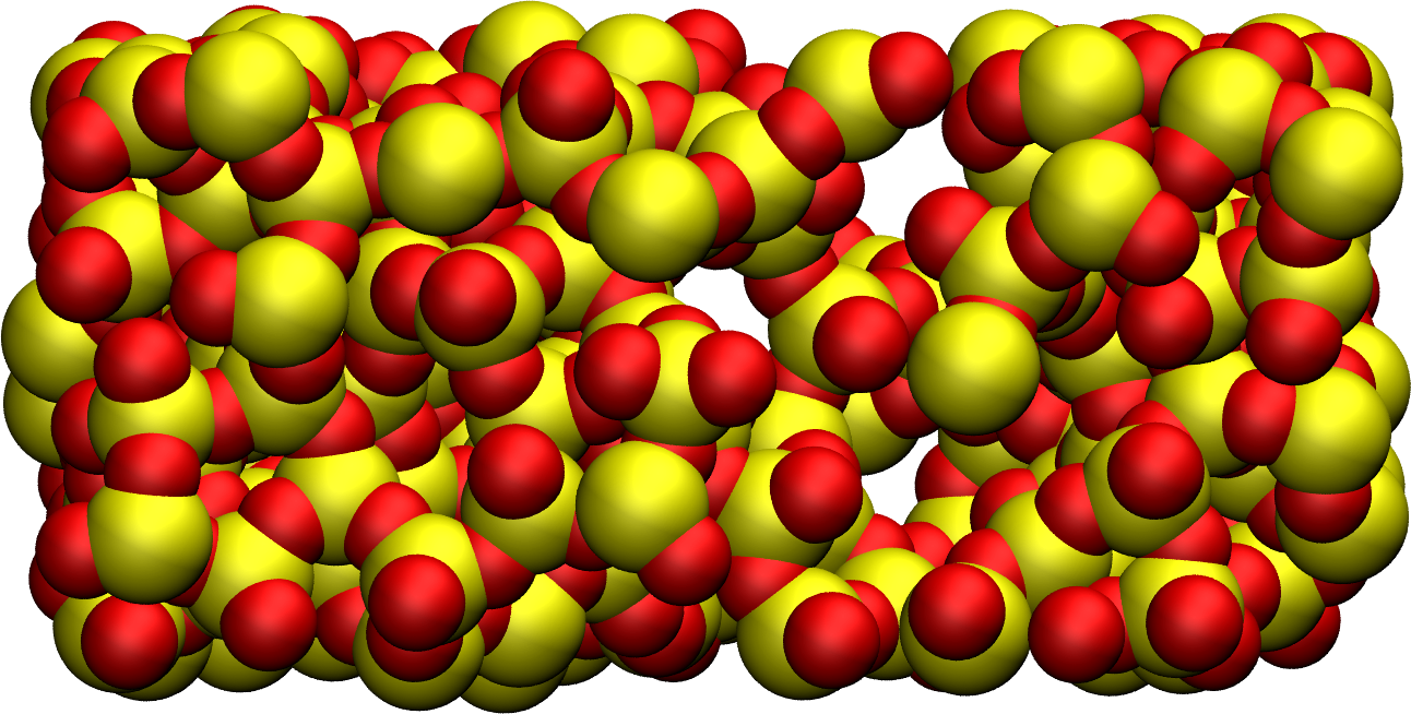
Figure: Block of silica after deformation. Silicon atoms are represented in yellow, and oxygen atoms in red. The crack was induced by the imposed deformation of the box along the \(x\)-axis (i.e., the horizontal axis).

Adding water

To add the water molecules to the silica, we will employ the Monte Carlo method in the grand canonical ensemble (GCMC). In short, the system is placed into contact with a virtual reservoir of a given chemical potential \(\mu\), and multiple attempts to insert water molecules at random positions are made. Each attempt is either accepted or rejected based on energy considerations. For further details, please refer to classical textbooks like Ref. [6].

Using hydrid potentials

The first particularly of our system is that it combines water and silica, which necessitates the use of two force fields: Vashishta (for \(\text{SiO}_2\)), and TIP4P (for water). Here, the TIP4P/2005 model is employed for the water [4].

Create a new file called gcmc.lmp, and copy the following lines into it:

units metal
boundary p p p
atom_style full
neighbor 1.0 bin
neigh_modify delay 1
pair_style hybrid/overlay vashishta lj/cut/tip4p/long OW HW OW-HW HW-OW-HW 0.1546 10
kspace_style pppm/tip4p 1.0e-5
bond_style harmonic
angle_style harmonic

If you are using LAMMPS-GUI

Open the gcmc.lmp file.

Combining the two force fields, Vashishta and TIP4P/2005, is achieved using the hybrid/overlay pair style. The PPPM solver [25] is specified with the kspace command, and is used to compute the long-range Coulomb interactions associated with tip4p/long. Finally, the style for the bonds and angles of the water molecules are defined; however, these specifications are not critical since TIP4P/2005 is a rigid water model.

The water molecule template called H2O.mol must be downloaded and located next to gcmc.lmp.

Before going further, we need to make a few changes to our data file. Currently, the cracking.data file includes only two atom types, but we require four. Copy the previously generated cracking.data, and name the duplicate cracking-mod.data. Make the following changes to the beginning of cracking-mod.data to ensure it matches the following format (with 4 atom types, 1 bond type, 1 angle type, the proper type labels, and four masses):

720 atoms
4 atom types
1 bond types
1 angle types

2 extra bond per atom
1 extra angle per atom
2 extra special per atom

-22.470320800269317 22.470320800269317 xlo xhi
-8.579178758211475 8.579178758211475 ylo yhi
-8.491043517346204 8.491043517346204 zlo zhi

Atom Type Labels

1 Si
2 O
3 OW
4 HW

Bond Type Labels

1 OW-HW

Angle Type Labels

1 HW-OW-HW

Masses

1 28.0855
2 15.9994
3 15.9994
4 1.008

Atoms # full

(...)

Doing so, we anticipate that there will be 4 atom types in the simulations, with the oxygens and hydrogens of \(\text{H}_2\text{O}\) having types OW and HW, respectively. There will also be 1 bond type (OW-HW) and 1 angle type (OW-HW-HW). The extra bond, extra angle, and extra special lines are here for memory allocation.

We can now proceed to complete the gcmc.lmp file by adding the system definition:

read_data cracking-mod.data
molecule h2omol H2O.mol
create_atoms 0 random 3 3245 NULL mol h2omol 4585 overlap 2.0 maxtry 50

group SiO type Si O
group H2O type OW HW

After reading the data file and defining the h2omol molecule from the H2O.mol file, the create_atoms command is used to include three water molecules in the system. Then, add the following pair_coeff (and bond_coeff and angle_coeff) commands to gcmc.lmp:

pair_coeff * * vashishta SiO.1990.vashishta Si O NULL NULL
pair_coeff * * lj/cut/tip4p/long 0 0
pair_coeff Si OW lj/cut/tip4p/long 0.0057 4.42
pair_coeff O OW lj/cut/tip4p/long 0.0043 3.12
pair_coeff OW OW lj/cut/tip4p/long 0.008 3.1589
pair_coeff HW HW lj/cut/tip4p/long 0.0 0.0
bond_coeff OW-HW 0 0.9572
angle_coeff HW-OW-HW 0 104.52

The force field Vashishta applies only to Si and O of \(\text{SiO}_2\), and not to the OW and HW of \(\text{H}_2\text{O}\), thanks to the NULL parameters used for atoms of types OW and HW. Pair coefficients for the lj/cut/tip4p/long potential are defined between O(\(\text{H}_2\text{O}\)) and between H(\(\text{H}_2\text{O}\)) atoms, as well as between O(\(\text{SiO}_2\))-O(\(\text{H}_2\text{O}\)) and Si(\(\text{SiO}_2\))-O(\(\text{H}_2\text{O}\)). Thus, the fluid-fluid and the fluid-solid interactions will be adressed with by the lj/cut/tip4p/long potential. The bond_coeff and angle_coeff commands set the OW-HW bond length to 0.9572 Å, and the HW-OW-HW angle to \(104.52^\circ\), respectively [4].

Add the following lines to gcmc.lmp as well:

variable oxygen atom type==label2type(atom,OW)
group oxygen dynamic all var oxygen
variable nO equal count(oxygen)

fix shak H2O shake 1.0e-5 200 0 b OW-HW a HW-OW-HW mol h2omol

The number of oxygen atoms from water molecules (i.e. the number of molecules) is calculated by the nO variable. The SHAKE algorithm is used to maintain the shape of the water molecules over time [34, 35].

Finally, let us create images of the system using dump image:

dump viz all image 250 myimage-*.ppm type type &
shiny 0.1 box no 0.01 view 180 90 zoom 3.4 size 1700 700
dump_modify viz backcolor white &
acolor Si yellow adiam Si 2.5 &
acolor O red adiam O 2 &
acolor OW cyan adiam OW 2 &
acolor HW white adiam HW 1

GCMC simulation

To prepare for the GCMC simulation, let us add the following lines into gcmc.lmp:

compute ctH2O H2O temp
compute_modify thermo_temp dynamic yes
compute_modify ctH2O dynamic yes
fix mynvt1 H2O nvt temp 300 300 0.1
fix_modify mynvt1 temp ctH2O
fix mynvt2 SiO nvt temp 300 300 0.1
timestep 0.001

Two different thermostats are used for \(\text{SiO}_2\) and \(\text{H}_2\text{O}\), respectively. Using separate thermostats is usually better when the system contains two separate species, such as a solid and a liquid. It is particularly important to use two thermostats here because the number of water molecules will fluctuate with time. The compute_modify command with the dynamic yes option for water is used to specify that the number of molecules will not be constant.

Finally, let us use the fix gcmc and perform the grand canonical Monte Carlo steps. Add the following lines into gcmc.lmp:

variable tfac equal 5.0/3.0
fix fgcmc H2O gcmc 100 100 0 0 65899 300 -0.5 0.1 mol h2omol tfac_insert ${tfac} shake shak full_energy pressure 100

The tfac_insert option ensures the correct estimate for the temperature of the inserted water molecules by taking into account the internal degrees of freedom. Here, 100 insertion and deletion attemps are made every 100 steps.

Note

At a pressure of \(p = 100\,\text{bar}\), the chemical potential of water vapor at \(T = 300\,\text{K}\) can be calculated using as \(\mu = \mu_0 + RT \ln (\frac{p}{p_0}),\) where \(\mu_0\) is the standard chemical potential (typically taken at a pressure \(p_0 = 1 \, \text{bar}\)), \(R = 8.314\, \text{J/mol·K}\) is the gas constant, \(T = 300\,\text{K}\) is the temperature.

Finally, let us print some information and run for 25 ps:

thermo 250
thermo_style custom step temp etotal v_nO f_fgcmc[3] f_fgcmc[4] f_fgcmc[5] f_fgcmc[6]

run 25000

Running this simulation using LAMMPS, one can see that the number of molecules is increasing progressively. When using the pressure argument, LAMMPS ignores the value of the chemical potential (here \(\mu = -0.5\,\text{eV}\), which corresponds roughly to ambient conditions, i.e. to a relative humidity \(\text{RH} \approx 50\,\%\) [44].) The large pressure value of 100 bars was chosen to ensure that some successful insertions of molecules would occur during the short duration of this simulation.

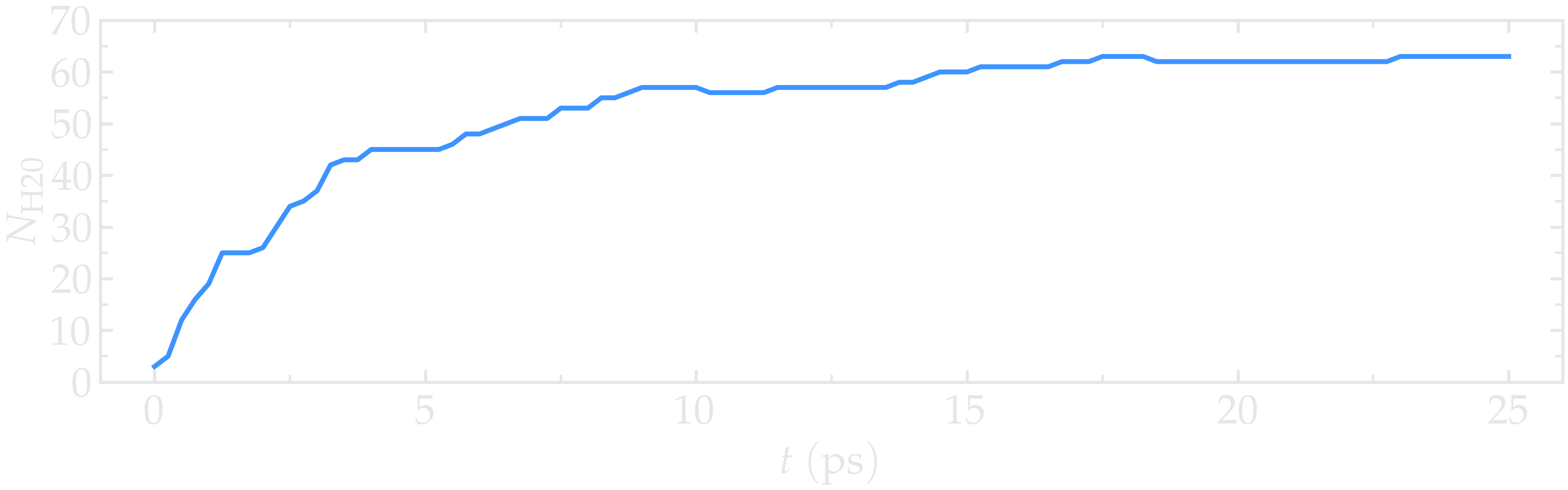
Figure: Number of water molecules, \(N_\text{H2O}\), as a function of time, \(t\).

After a few GCMC steps, the number of molecules starts increasing. Once the crack is filled with water molecules, the total number of molecules reaches a plateau. The final number of molecules depends on the imposed pressure, temperature, and the interaction between water and silica (i.e. its hydrophilicity). Note that GCMC simulations of such dense phases are usually slow to converge due to the very low probability of successfully inserting a molecule. Here, the short simulation duration was made possible by the use of a high pressure.

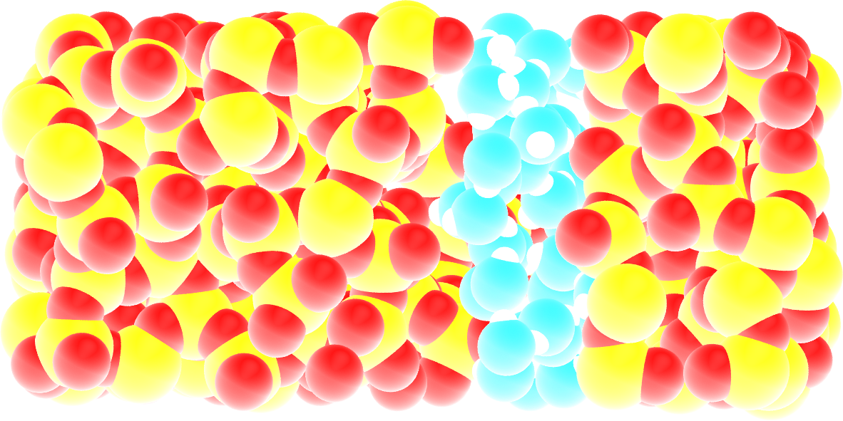
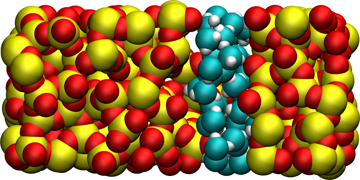
Figure: Snapshot of the silica system after the adsorption of water molecules. The oxygen atoms of the water molecules are represented in cyan, the silicon atoms in yellow, and the oxygen atoms of the solid in red.

Cite

You can access the input scripts and data files that are used in these tutorials from a dedicated Github repository. This repository also contains the full solutions to the exercises.

Going further with exercises

Mixture adsorption

Adapt the existing script and insert both \(\text{CO}_2\) molecules and water molecules within the silica crack using GCMC. Download the CO2 template. The parameters for the \(\text{CO}_2\) molecule are the following:

pair_coeff 5 5 lj/cut/tip4p/long 0.0179 2.625854
pair_coeff 6 6 lj/cut/tip4p/long 0.0106 2.8114421
bond_coeff 2 46.121 1.17
angle_coeff 2 2.0918 180

The atom of type 5 is an oxygen of mass 15.9994, and the atom of type 6 is a carbon of mass 12.011.

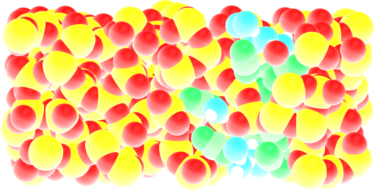
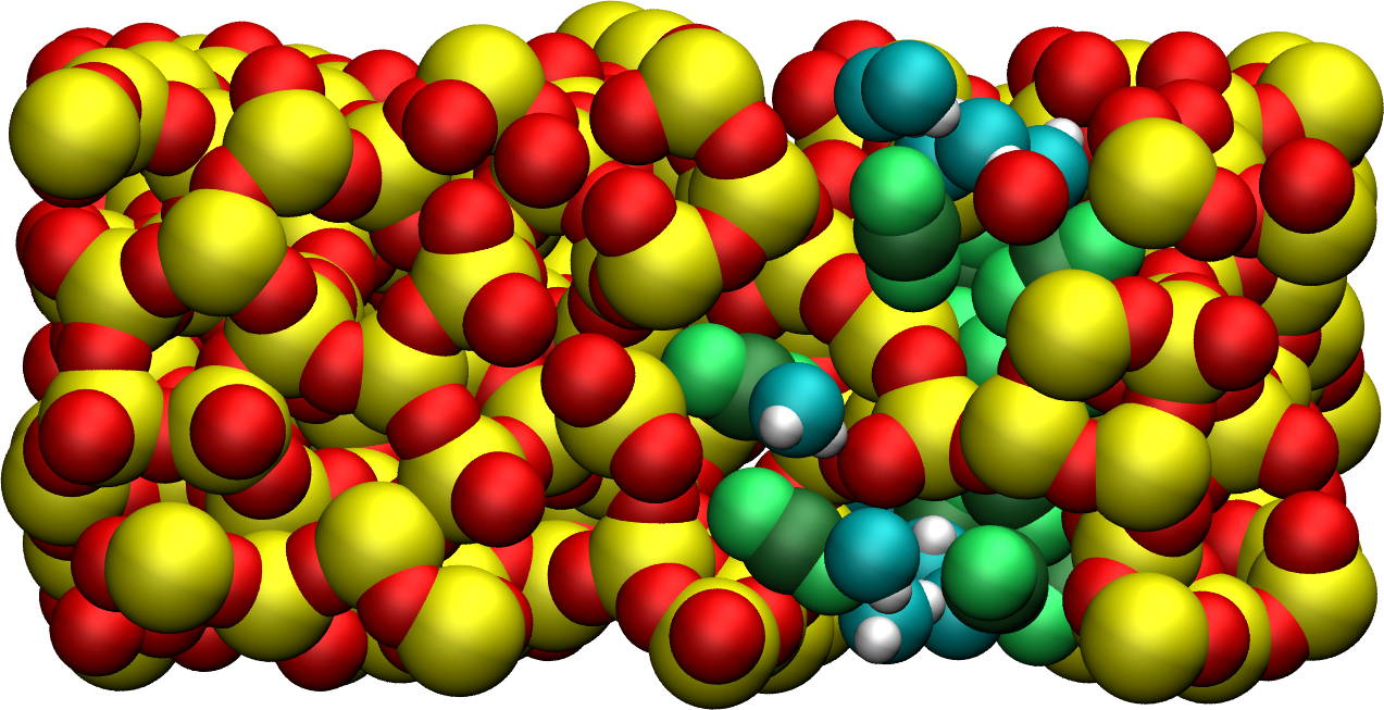
Figure: Cracked silica with adsorbed water and \(\text{CO}_2\) molecules (in green).

Adsorb water in ZIF-8 nanopores

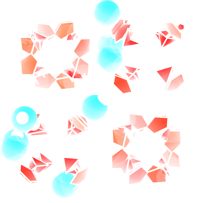
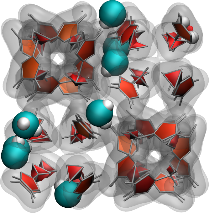
Use the same protocol as the one implemented in this tutorial to add water molecules to a Zif-8 nanoporous material. A snapshot of the system with a few water molecules is shown on the right.

Download the initial Zif-8 structure, the parameters file, and this new water template. The ZIF-8 structure is made of 7 atom types (C1, C2, C3, H2, H3, N, Zn), connected by bonds, angles, dihedrals, and impropers. It uses the same pair_style as water, so there is no need to use hybrid pair_style. Your input file should start like this:

units real
atom_style full
boundary p p p
bond_style harmonic
angle_style harmonic
dihedral_style charmm
improper_style harmonic

pair_style lj/cut/tip4p/long 1 2 1 1 0.105 14.0
kspace_style pppm/tip4p 1.0e-5

special_bonds lj 0.0 0.0 0.5 coul 0.0 0.0 0.833

An important note: here, water occupies the atom types 1 and 2, instead of 3 and 4 in the case of SiO2 from the main section of the tutorial.