Pulling on a carbon nanotube
Stretching a carbon nanotube until it breaks
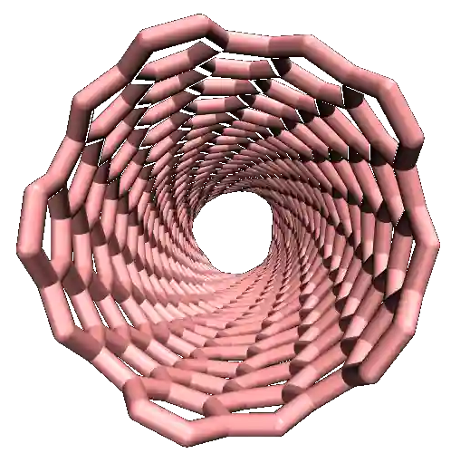
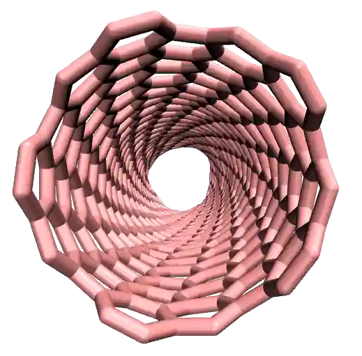
In this tutorial, the system of interest is a small, single-walled carbon nanotube (CNT) in an empty box. The CNT is strained by imposing a constant velocity on the edge atoms. To illustrate the difference between conventional and reactive force fields, this tutorial is divided into two parts: in the first part, a conventional molecular force field (called OPLS-AA [1]) is used and the functional form of the bonded potential ensures that the bonds between the atoms of the CNT are unbreakable. In the second part, a reactive, many-body, force field (called AIREBO [2]) is used, which allows chemical bonds to break under large strain.
If you are completely new to LAMMPS, we recommend that you follow this tutorial on a simple Lennard-Jones fluid first.
Cite
If you find these tutorials useful, you can cite A Set of Tutorials for the LAMMPS Simulation Package [Article v1.0] by Simon Gravelle, Cecilia M. S. Alvares, Jacob R. Gissinger, and Axel Kohlmeyer, published in LiveCoMS, 6(1), 3037 (2025) [14].
This tutorial is compatible with the 22Jul2025 LAMMPS version.
Unbreakable bonds
With most conventional molecular force fields, the chemical bonds between
atoms are defined at the start of the simulation and remain fixed, regardless
of the forces applied to the atoms. In this tutorial, these bonds are
explicitly specified in the .data file, which is read using the read_data command (see below).
Bonds are typically modeled as springs following Hooke’s law
with equilibrium distances \(r_0\), force constants \(k_\text{b}\),
and bond potential energy \(U_\text{b} = k_\text{b} \left( r - r_0 \right)^2\).
Additionally, angular and dihedral constraints are often imposed to preserve the
molecular structure by maintaining the relative orientations of neighboring atoms.
The LAMMPS input
To begin this tutorial, if you are using LAMMPS–GUI, select
Start Tutorial 2 from the Tutorials menu of LAMMPS-GUI
and follow the instructions. This will select a folder, create one if
necessary, and place several files into it. The initial input file,
set up for a single-point energy calculation, will also be loaded into
the editor under the name unbreakable.lmp. Additional files
are a data file containing the CNT topology and geometry, named
unbreakable.data, a parameters file named unbreakable.inc, as well as
the scripts required for the second part of the tutorial.
units real
atom_style molecular
boundary f f f

pair_style lj/cut 14.0
bond_style harmonic
angle_style harmonic
dihedral_style opls
improper_style harmonic
special_bonds lj 0.0 0.0 0.5

read_data unbreakable.data
include unbreakable.inc

run 0 post no
If you are not using LAMMPS-GUI
Create a folder if needed and place the initial input file, unbreakable.lmp, into it. Then, open the file in a text editor of your choice, and copy the previous lines into it.
The chosen unit system is real (therefore distances are in
Ångströms (Å), times in femtoseconds (fs), and energies in (kcal/mol)), the
atom_style is molecular (therefore atoms are point
particles that can form bonds with each other), and the boundary
conditions are fixed. The boundary conditions do not matter here, as
the box boundaries were placed far from the CNT. Just like in the
previous tutorial, Lennard-Jones fluid,
the pair style is lj/cut (i.e. a Lennard-Jones potential with
cutoff) and its cutoff is set to 14 Å, which means that only the
atoms closer than this distance interact through the Lennard-Jones
potential.
Looking for help with your project ?
Get guidance for your LAMMPS simulations and receive personalized advice for your project.
The bond_style, angle_style, dihedral_style, and improper_style
commands specify the different potentials used to constrain the relative
positions of the atoms. The special_bonds command sets the weighting factors
for the Lennard-Jones interactions between atoms sitting one,
two, or three bonds away from each other, respectively. This is done for
convenience when parameterizing the force constants for bonds, angles, and
so on. By excluding the non-bonded (Lennard-Jones) interactions for
these pairs, those interactions do not need to be considered when determining
the force constants.
The read_data command imports the unbreakable.data
file that should be downloaded next to unbreakable.lmp. This file contains information about the box size, atom positions,
as well as the identity of the atoms that are linked by bonds, angles,
dihedrals, and impropers interactions. It was created using VMD and TopoTools
[21].
Note
Bonds, angles, dihedrals, and impropers in LAMMPS are assigned types and IDs, just like atoms.
The ID uniquely identifies each interaction instance, while the type determines which parameters
(from the bond_coeff, angle_coeff, etc. commands) are applied.
In this tutorial, these types and IDs are specified in the .data file and
read by the read_data command.
Note
The format details of the different sections in a data file change with different
settings. In particular, the Atoms section may have a different number of
columns, or the columns may represent different properties when the atom_style
is changed. To help users, LAMMPS and tools like VMD and TopoTools will add a
comment (here # molecular) to the Atoms header line in the data files that
indicates the intended atom_style. LAMMPS will print a warning when the chosen
atom style does not match what is written in that comment.
The .data file does not contain any sections with potential parameters; thus, we need to specify the parameters of both the bonded and non-bonded potentials. The parameters we use are taken from the OPLS-AA (Optimized Potentials for Liquid Simulations-All-Atom) force field [1], and are given in a separate unbreakable.inc file (also downloaded during the tutorial setup). This file - that must be placed next to unbreakable.lmp - contains the following lines:
pair_coeff 1 1 0.066 3.4
bond_coeff 1 469 1.4
angle_coeff 1 63 120
dihedral_coeff 1 0 7.25 0 0
improper_coeff 1 5 180
The pair_coeff command sets the parameters for non-bonded
Lennard-Jones interactions atom type 1 to
\(\epsilon_{11} = 0.066 \, \text{kcal/mol}\) and
\(\sigma_{11} = 3.4 \, \text{Å}\). The bond_coeff provides
the equilibrium distance \(r_0 = 1.4 \, \text{Å}\) and the
spring constant \(k_\text{b} = 469 \, \text{kcal/mol/Å}^2\) for the
harmonic potential imposed between two neighboring carbon atoms. The potential
is given by \(U_\text{b} = k_\text{b} ( r - r_0)^2\). The
angle_coeff gives the equilibrium angle \(\theta_0\) and
constant for the potential between three neighboring atoms :
\(U_\theta = k_\theta ( \theta - \theta_0)^2\). The
dihedral_coeff and improper_coeff define the potentials
for the constraints between 4 atoms.
Note
Rather than copying the contents of the file into the input, we
incorporate it using the include command. Using include allows
us to conveniently reuse the parameter settings
in other inputs or switch them with others. This will become more general
when using type labels, which is shown in the next
tutorial [3].
Prepare the initial state
In this tutorial, a deformation will be applied to the CNT by displacing
the atoms located at its edges. To achieve this, we will first isolate the
atoms at the two edges and place them into groups named rtop and
rbot. Add the following lines to unbreakable.lmp,
just before the run 0 command:
group carbon_atoms type 1
variable xmax equal bound(carbon_atoms,xmax)-0.5
variable xmin equal bound(carbon_atoms,xmin)+0.5
region rtop block ${xmax} INF INF INF INF INF
region rbot block INF ${xmin} INF INF INF INF
region rmid block ${xmin} ${xmax} INF INF INF INF
The first command includes all the atoms of type 1 (i.e. all the atoms here)
in a group named carbon_atoms.
The variable \(x_\text{max}\) corresponds to the coordinate of the
last atoms along \(x\) minus \(0.5 \, \text{Å}\), and \(x_\text{min}\) to the coordinate
of the first atoms along \(x\) plus \(0.5 \, \text{Å}\). Then, three regions are defined,
corresponding to the following: \(x < x_\text{min}\) (rbot, for region
bottom), \(x_\text{min} > x > x_\text{max}\) (rmid, for region middle),
and \(x > x_\text{max}\) (rtop, for region top).
Note
So far, variables have been referenced dynamically during the run using
the v_ prefix, which evaluates the variable as it evolves over time.
Here, a dollar sign ($) is used to reference the variable at the time the script is read.
Finally, let us define 3 groups of atoms corresponding to the atoms
in each of the 3 regions by adding to unbreakable.lmp
just before the run 0 command:
group cnt_top region rtop
group cnt_bot region rbot
group cnt_mid region rmid
set group cnt_top mol 1
set group cnt_bot mol 2
set group cnt_mid mol 3
With the three set commands, we assign unique, otherwise unused
molecule IDs to atoms in those three groups. A molecule ID is an
integer that groups atoms into a molecule for bookkeeping purposes, and can be
useful for tracking and post-processing. We will use this IDs later to
assign different colors to these groups of atoms.
Run the simulation using LAMMPS. The number of atoms in each group is given in
the Output window. It is an important check to make sure that the number
of atoms in each group corresponds to what is expected, as shown here:
700 atoms in group carbon_atoms
10 atoms in group cnt_top
10 atoms in group cnt_bot
680 atoms in group cnt_mid
Finally, to start from a less ideal state and create a system with some defects,
let us randomly delete a small fraction of the carbon atoms. To avoid deleting
atoms that are too close to the edges, let us define a new region named rdel
that starts at \(2 \, \text{Å}\) from the CNT edges:
variable xmax_del equal ${xmax}-2
variable xmin_del equal ${xmin}+2
region rdel block ${xmin_del} ${xmax_del} INF INF INF INF
group rdel region rdel
delete_atoms random fraction 0.02 no rdel NULL 2793 bond yes
The delete_atoms command randomly deletes \(2\,\%\) of the atoms from
the rdel group, here about 10 atoms.
The molecular dynamics
Let us give an initial temperature to the atoms of the group cnt_mid
by adding the following commands to unbreakable.lmp:
reset_atoms id sort yes
velocity cnt_mid create 300 48455 mom yes rot yes
Re-setting the atom IDs is necessary before using the velocity command
when atoms were deleted, which is done here with the reset_atoms command.
The velocity command assigns random initial velocities to the atoms of the middle
group cnt_mid from a uniform distribution, ensuring an initial temperature
of \(T = 300\,\text{K}\) for these atoms.
Let us specify the thermalization and the dynamics of the system. Add the following lines into unbreakable.lmp:
fix mynve1 cnt_top nve
fix mynve2 cnt_bot nve
fix mynvt cnt_mid nvt temp 300 300 100
The fix nve commands are applied to the atoms of cnt_top and
cnt_bot, respectively, and will ensure that the positions of the atoms
from these groups are recalculated at every step. The fix nvt does the
same for the cnt_mid group, while also applying a Nosé-Hoover thermostat
with desired temperature of 300 K [22, 23].
Note
The Nosé-Hoover thermostat only controls the temperature of the atoms
belonging to the specified cnt_mid group. Atoms outside this group are not affected.
To immobilize the motion of the atoms at the edges, let us add the following commands to unbreakable.lmp:
fix mysf1 cnt_top setforce 0 0 0
fix mysf2 cnt_bot setforce 0 0 0
velocity cnt_top set 0 0 0
velocity cnt_bot set 0 0 0
The two setforce commands cancel the forces applied on the atoms of the
two edges, respectively. The cancellation of the forces is done at every step,
and along all 3 directions of space, \(x\), \(y\), and \(z\), due to the use of
0 0 0. Although the forces on these atoms is set to zero,
the fix still stores the forces acting on the group before
cancellation, which can later be extracted for analysis (see below).
The two velocity commands set the initial velocities
along \(x\), \(y\), and \(z\) to 0 for the atoms of cnt_top and
cnt_bot, respectively. As a consequence of these last four commands,
the atoms of the edges will remain immobile during the simulation (or at least
they would if no other command was applied to them).
Note
The velocity set command adjusts the velocities of a
group of atoms immediately but has no effect during
the simulation. When velocity set is used in combination with
setforce 0 0 0, as is the case here, the atoms won’t feel any force during the entire simulation.
According to the Newton equation, no force means no acceleration, meaning that the initial velocity
will persist during the entire simulation, thus producing a constant velocity motion or no motion at all.
Outputs
Next, to measure the strain and stress applied to the CNT, let us create a variable for the distance \(L_\text{cnt}\) between the two edges, as well as a variable \(F_\text{cnt}\) for the force applied on the edges:
variable Lcnt equal xcm(cnt_top,x)-xcm(cnt_bot,x)
variable Fcnt equal f_mysf1[1]-f_mysf2[1]
Here, the force is extracted from the fixes mysf1 and mysf2
using f_ , similarly to the use of v_ to call a variable,
and c_ to call a compute, as seen in Lennard-Jones fluid.
Let us also add a dump image command to visualize the system every 500 steps:
dump viz all image 500 myimage-*.ppm element type size 1000 400 zoom 6 shiny 0.3 fsaa yes &
    bond atom 0.8 view 0 90 box no 0.0 axes no 0.0 0.0
dump_modify viz pad 9 backcolor white adiam 1 0.85 bdiam 1 1.0
Let us run a small equilibration step to bring the system to the required
temperature before applying any deformation. Replace the run 0 post no
command in unbreakable.lmp with the following lines:
compute Tmid cnt_mid temp
thermo 100
thermo_style custom step temp etotal v_Lcnt v_Fcnt
thermo_modify temp Tmid line yaml

timestep 1.0
run 5000
With the thermo_modify command, we specify to LAMMPS that the
temperature \(T_\mathrm{mid}\) of the middle group, cnt_mid,
must be outputted, instead of the temperature of the entire system.
This choice is motivated by the presence of frozen parts with an effective temperature of \(0~\text{K}\),
which makes the average temperature of the entire system less relevant.
The thermo_modify command also imposes the use of the YAML format that can easily be read by
Python (see below).
Let us impose a constant velocity deformation on the CNT
by combining the velocity set command with previously defined
fix setforce. Add the following lines in the unbreakable.lmp
file, right after the last run 5000 command:
velocity cnt_top set 0.0005 0 0
velocity cnt_bot set -0.0005 0 0

run 10000
The chosen velocity for the deformation is \(100\,\text{m/s}\), or \(0.001\,\text{Å/fs}\). Run the simulation using LAMMPS. As can be seen from the variable \(L_\text{cnt}\), the length of the CNT increases linearly over time for \(t > 5\,\text{ps}\), as expected from the imposed constant velocity. What you observe in the Slide Show windows should resemble the figure below.
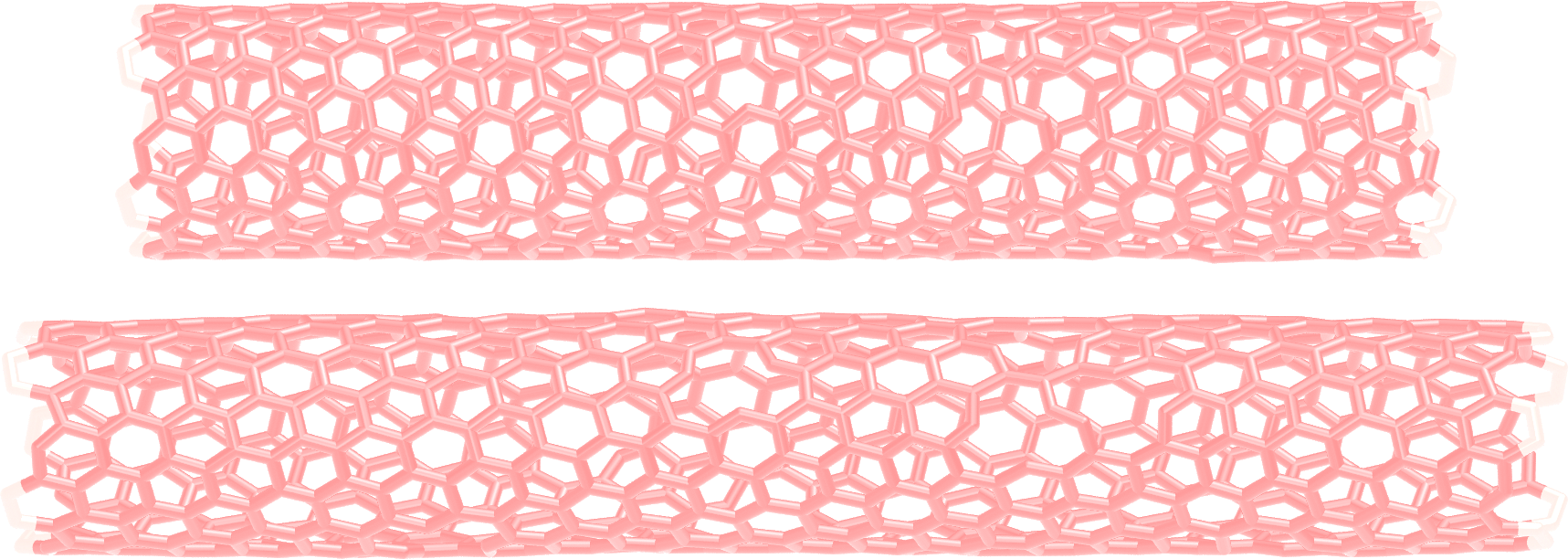
The unbreakable CNT before (top) and after deformation (bottom).
The total energy of the system shows a non-linear increase with \(t\) once the deformation starts, which is expected from the typical dependency of bond energy with bond distance, \(U_\text{b} = k_\text{b} \left( r - r_0 \right)^2\).
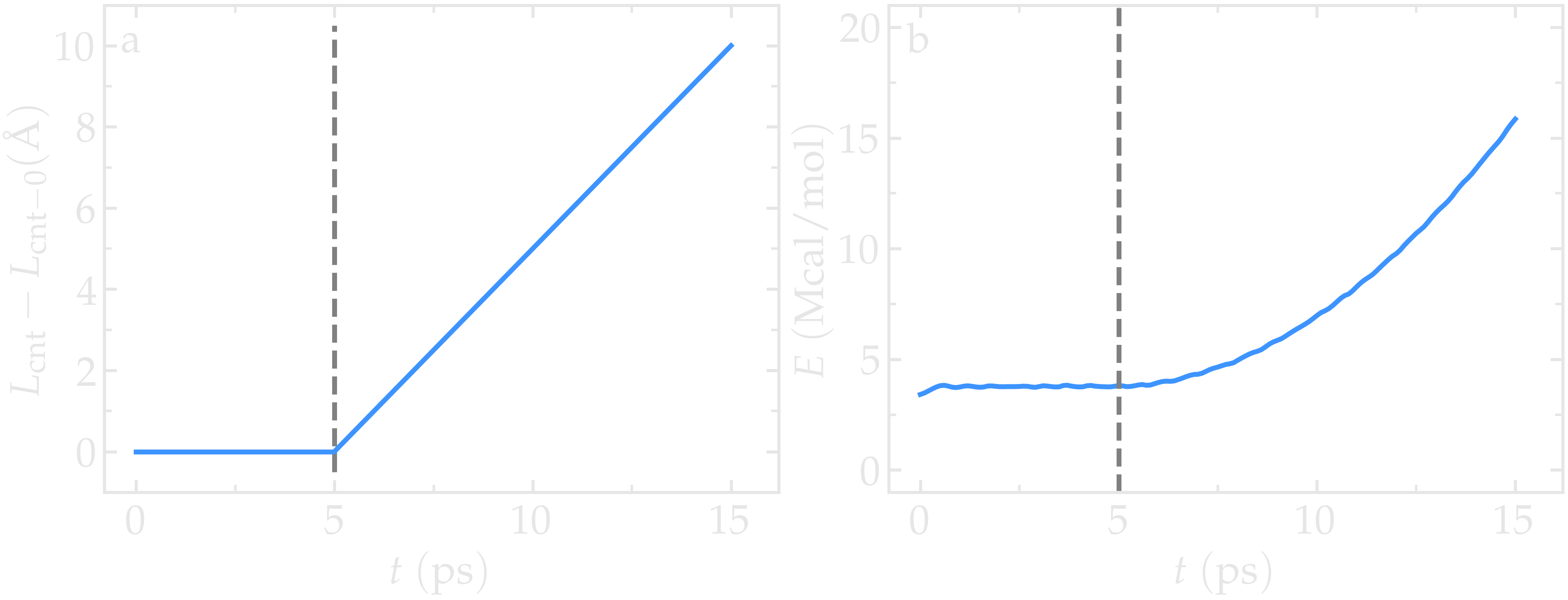
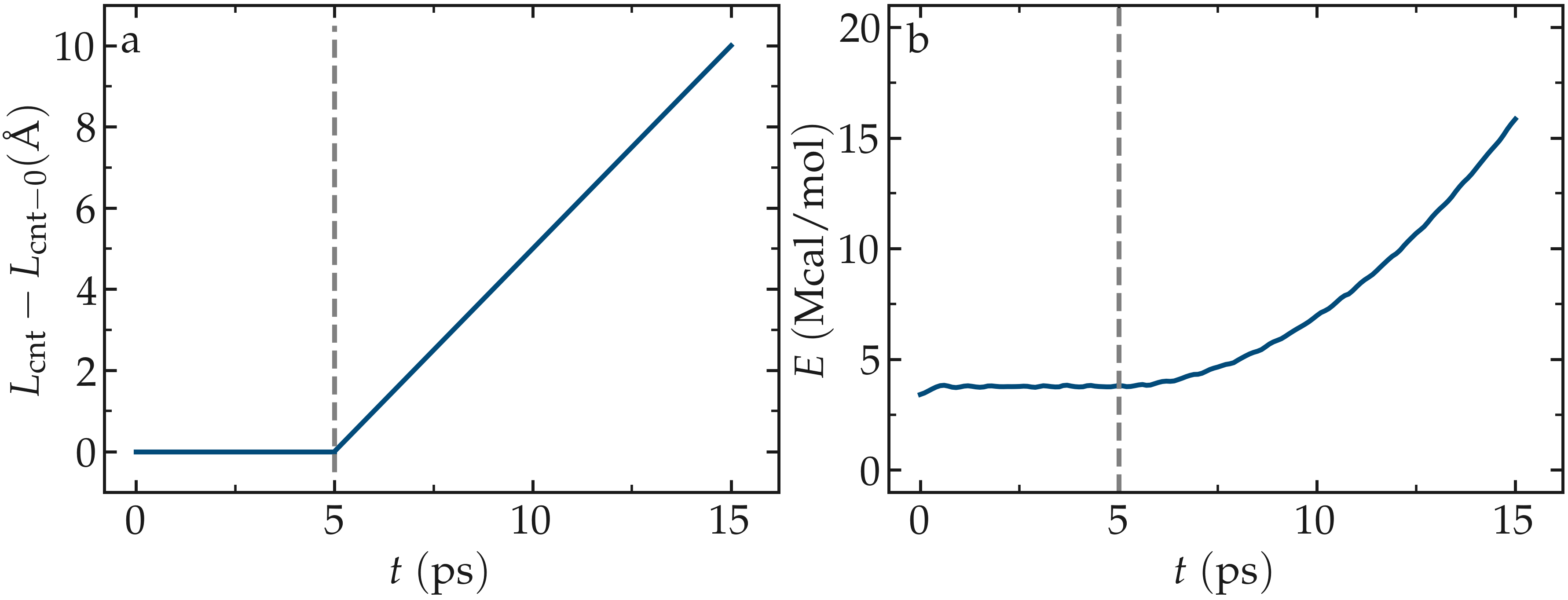
Figure: a) Evolution of the length \(L_\text{cnt}\) of the CNT with time. The CNT starts deforming at \(t = 5\,\text{ps}\), and \(L_\text{cnt-0}\) is the CNT initial length. b) Evolution of the total energy \(E\) of the system with time \(t\). Here, the potential is OPLS-AA, and the CNT is unbreakable. The orange line shows the raw data, and the blue line represents a time-averaged curve.
Importing YAML log file into Python
Let us import the simulation data into Python, and generate a stress-strain curve. Here, the stress is defined as \(F_\text{cnt}/A_\text{cnt}\), where \(A_\text{cnt} = \pi r_\text{cnt}^2\) is the surface area of the CNT, and \(r_\text{cnt}=5.2\,\text{Å}\) the CNT radius. The strain is defined as \((L_\text{cnt}-L_\text{cnt-0})/L_\text{cnt-0}\), where \(L_\text{cnt-0}\) is the initial CNT length.
Right-click inside the Output window, and select
Export YAML data to file. Call the output unbreakable.yaml, and save
it within the same folder as the input files, where a Python script named unbreakable-yaml-reader.py should also
be located. When executed using Python, this .py file first imports
the unbreakable.yaml file. Then, a certain pattern is
identified and stored as a string character named docs. The string is
then converted into a list, and \(F_\text{cnt}\) and \(L_\text{cnt}\)
are extracted. The stress and strain are then calculated, and the result
is saved in a data file named unbreakable.dat using
the NumPy savetxt function. thermo[0] can be used to access the
information from the first minimization run, and thermo[1] to access the
information from the second MD run. The data extracted from
the unbreakable.yaml file can then be used to plot the stress-strain curve.
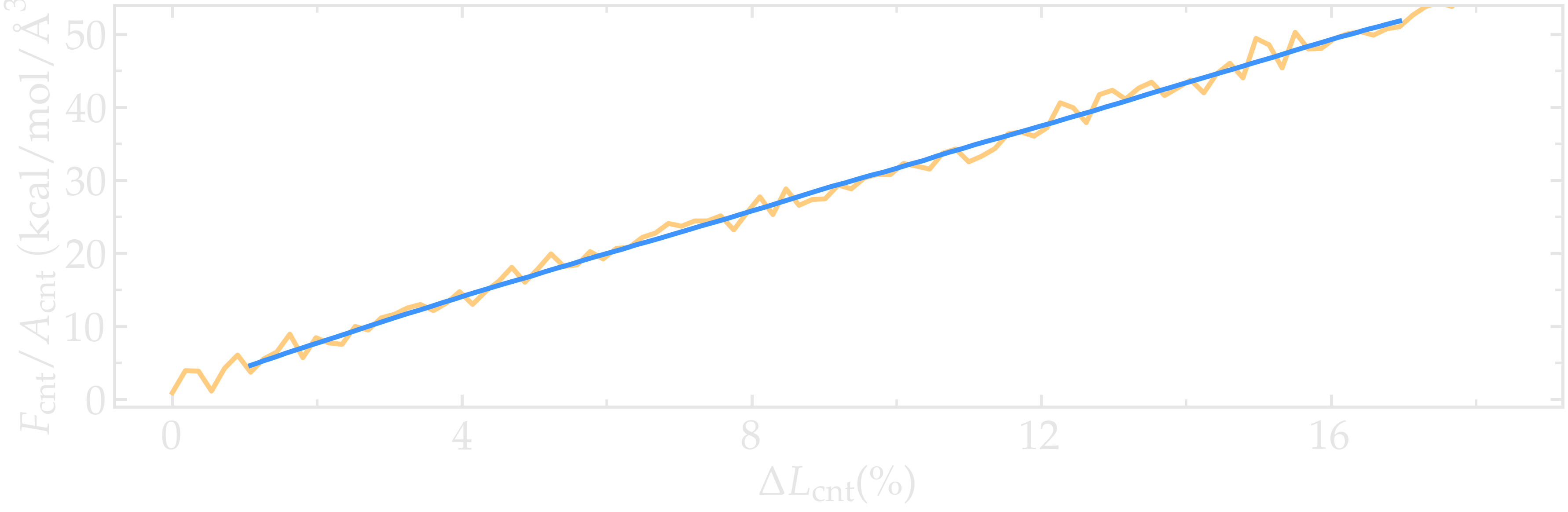
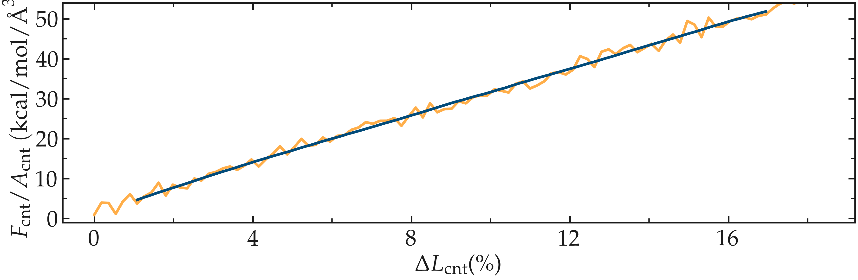
Figure: Stress applied on the CNT during deformation, \(F_\text{cnt}/A_\text{cnt}\), where \(F_\text{cnt}\) is the force and \(A_\text{cnt}\) the CNT surface area, as a function of the strain, \(\Delta L_\text{cnt} = (L_\text{cnt}-L_\text{cnt-0})/L_\text{cnt-0}\), where \(L_\text{cnt}\) is the CNT length and \(L_\text{cnt-0}\) the CNT initial length. Here, the potential is OPLS-AA, and the CNT is unbreakable. The orange line shows the raw data, and the blue line represents a time-averaged curve.
Breakable bonds
When using a conventional molecular force field, as we have just done, the bonds between the atoms are non-breakable. Let us perform a similar simulation and deform a small CNT again, but this time with a reactive force field that allows bonds to break if the applied deformation is large enough.
Input file initialization
Open the input named breakable.lmp
that should have been downloaded next to unbreakable.lmp during
the tutorial setup. There are only a few differences with the previous
input. First, the AIREBO force field requires the metal units
setting instead of real for OPLS-AA. A second difference is
the use of atom_style atomic instead of
molecular, since no explicit bond information is required with
AIREBO. The following commands are setting up the AIREBO force field:
pair_style airebo 3.0
pair_coeff * * CH.airebo C
Here, CH.airebo is the file containing the parameters for AIREBO, and must be placed next to breakable.lmp.
Note
The AIREBO force field is a many-body
potential, where interactions are not only between pairs of atoms,
but also triples and quadruples representing angle and dihedral
interactions. This means that there are different rules for the
pair_coeff command: there must be only one command that
covers all permutations of atom types by using two ‘*’ wildcards.
After the potential file follows a list of elements. These element
names are used to look up the parameter sets in the potential file.
There must be a list with as many elements as atom types following
the filename. In our system, there is only one atom type (1), which is
mapped to the element ‘C’ in the pair_coeff command.
Which elements are supported is determined by the contents of the
potential file.
Note
With metal units, time values are in units of picoseconds
(\(10^{-12}\,\text{s}\)) instead of femtoseconds (\(10^{-15}\,\text{s}\)) in the case of
real units. It is important to keep this in mind when
setting parameters that are expressed in units containing time, such as
the timestep or the time constant of a thermostat, or velocities.
Since bonds, angles, and dihedrals do not need to be explicitly set when using AIREBO, some simplification must be made to the .data file. The new .data file is named breakable.data and must be placed within the same folder as the input file. Just like unbreakable.data, the breakable.data contains the information required for placing the atoms in the box, but no bond/angle/dihedral information. Another difference between the unbreakable.data and breakable.data files is that, here, a larger distance of \(120~\text{Å}\) was used for the box size along the \(x\)-axis, to allow for larger deformation of the CNT.
Start the simulation
Here, let us perform a similar deformation as the previous one.
In breakable.lmp, replace the run 0 post no line with:
fix mysf1 cnt_bot setforce 0 0 0
fix mysf2 cnt_top setforce 0 0 0
velocity cnt_bot set 0 0 0
velocity cnt_top set 0 0 0

variable Lcnt equal xcm(cnt_top,x)-xcm(cnt_bot,x)
variable Fcnt equal f_mysf1[1]-f_mysf2[1]

dump viz all image 500 myimage.*.ppm type type size 1000 400 zoom 4 shiny 0.3 adiam 1.5 box no 0.01 view 0 90 shiny 0.1 fsaa yes
dump_modify viz pad 5 backcolor white acolor 1 gray

compute Tmid cnt_mid temp
thermo 100
thermo_style custom step temp etotal v_Lcnt v_Fcnt
thermo_modify temp Tmid line yaml

timestep 0.0005
run 10000
Note the relatively small timestep of \(0.0005\),ps (\(= 0.5\),fs) used. Reactive force fields like AIREBO usually require a smaller timestep than conventional ones. When running breakable.lmp with LAMMPS, you can see that the temperature deviates from the target temperature of \(300\,\text{K}\) at the start of the equilibration, but that after a few steps, it reaches the target value.
Note
Bonds cannot be displayed by the dump image when using
the atom_style atomic, as it contains no bonds. A
tip for displaying bonds with the
present system using LAMMPS is provided at the end of the tutorial.
You can also use external tools like VMD or OVITO (see the
tip for tutorial 3).
Launch the deformation
After equilibration, let us set the velocity of the edges equal to \(75~\text{m/s}\) (or \(0.75~\text{Å/ps}\)) and run for a longer duration than previously. Add the following lines into breakable.lmp:
velocity cnt_top set 0.75 0 0
velocity cnt_bot set -0.75 0 0

run 30000
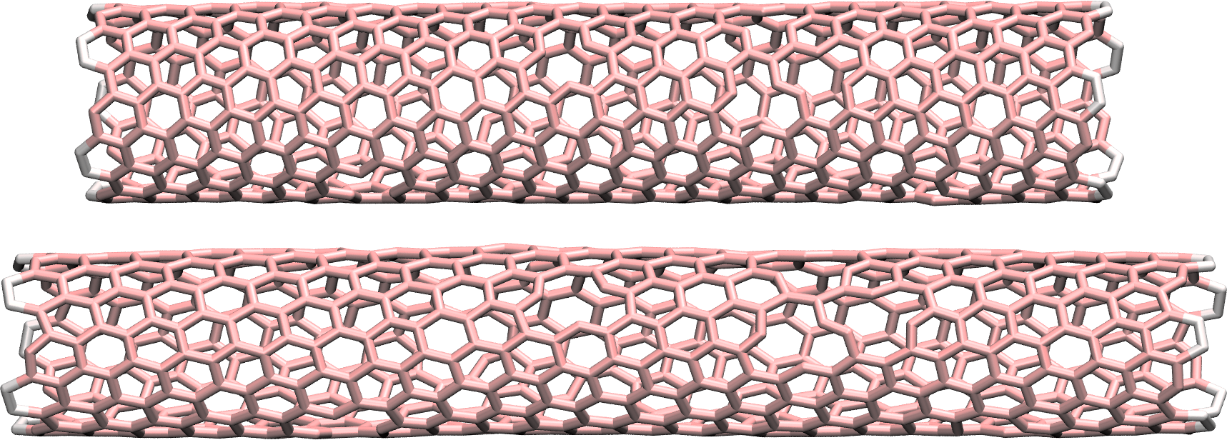
Run the simulation. Some bonds are expected to break before the end of the simulation.
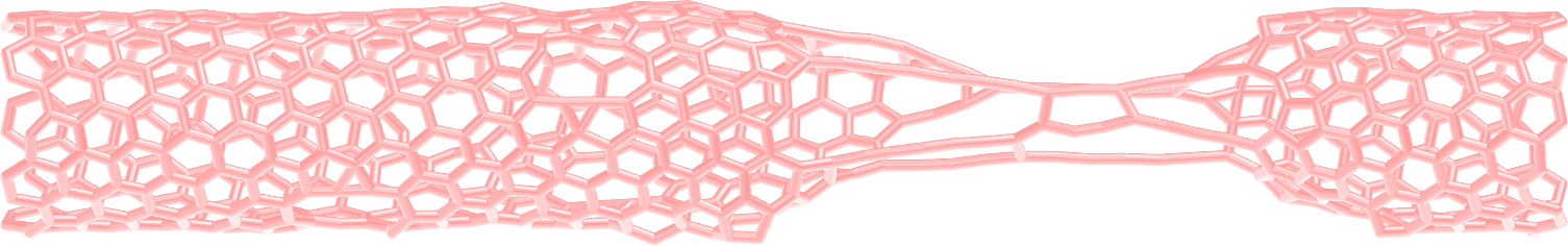
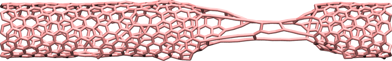
Figure: Figure: CNT with broken bonds. This image was generated using
VMD [12] DynamicBonds representation.
Looking at the evolution of the energy, one can see that the total energy \(E\) is initially increasing with the deformation. When bonds break, the energy relaxes abruptly, as can be seen near \(t=32~\text{ps}\). Using a similar script as previously, i.e., unbreakable-yaml-reader.py, import the data into Python and generate the stress-strain curve. The stress-strain curve reveals a linear (elastic) regime where \(F_\text{cnt} \propto \Delta L_\text{cnt}\) for \(\Delta L_\text{cnt} < 5\,\%\), and a non-linear (plastic) regime for \(5\,\% < \Delta L_\text{cnt} < 25\,\%\).
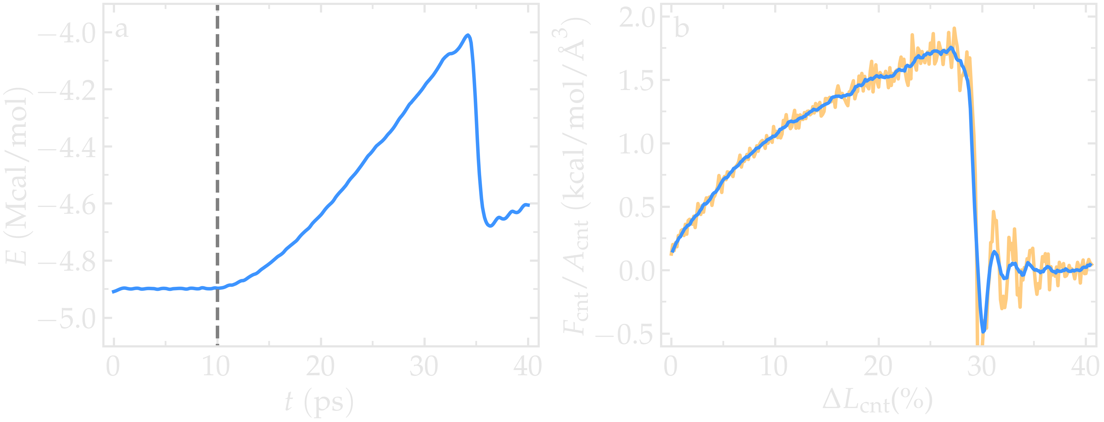
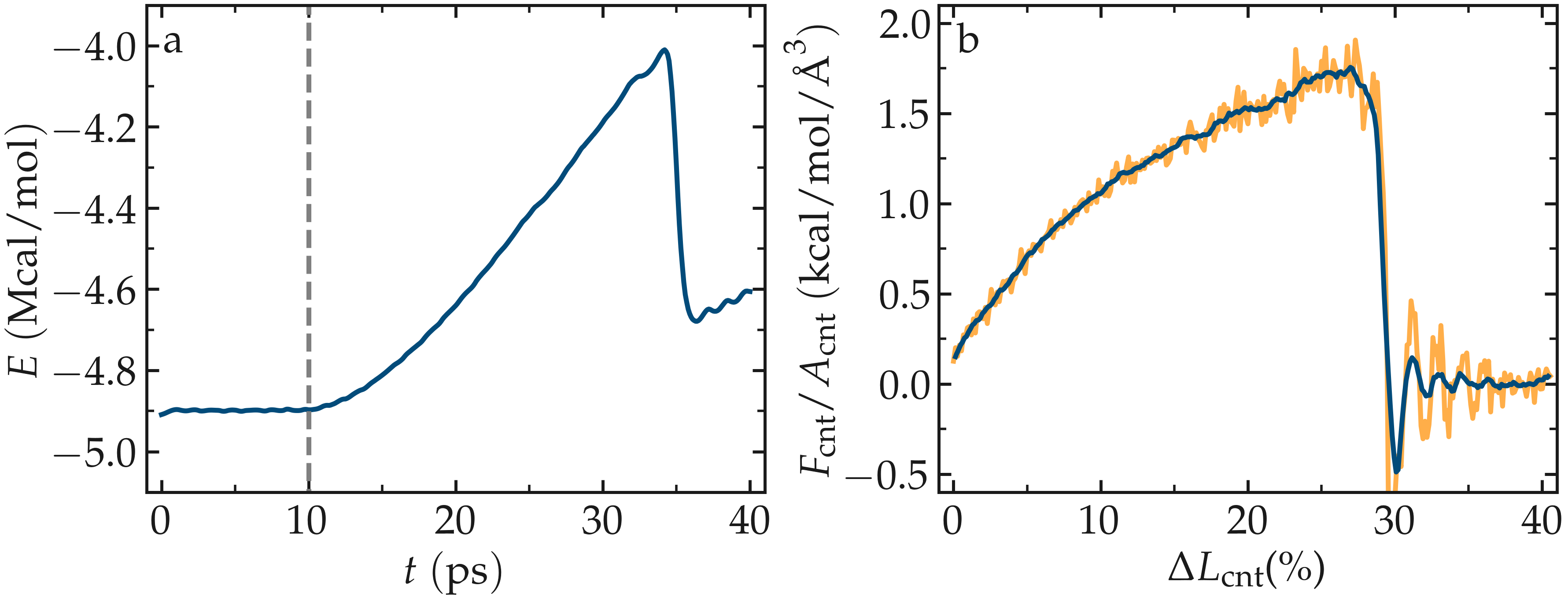
Figure: Figure: a) Evolution of the total energy \(E\) of the CNT with time \(t\). b) Stress applied on the CNT during deformation, \(F_\text{cnt}/A_\text{cnt}\), where \(F_\text{cnt}\) is the force and \(A_\text{cnt}\) the CNT surface area, as a function of the strain, \(\Delta L_\text{cnt} = (L_\text{cnt}-L_\text{cnt-0}/L_\text{cnt-0})\), where \(L_\text{cnt}\) is the CNT length and \(L_\text{cnt-0}\) the CNT initial length. Here, the potential is AIREBO, and the CNT is breakable. The orange line shows the raw data, and the blue line represents a time-averaged curve.
Tip: bonds representation with AIREBO
In the input file named breakable-with-tip.lmp,,
which is an alternate solution for breakable.lmp, a trick is
used to represent bonds while using AIREBO. A detailed explanation of
the script is beyond the scope of the present tutorial. In short, the
trick is to use AIREBO with the molecular atom style, and use
the fix bond/break and fix bond/create/angle commands
to update the status of the bonds during the simulation:
fix break all bond/break 1000 1 2.5
fix form all bond/create/angle 1000 1 1 2.0 1 aconstrain 90.0 180
This hack works because AIREBO does not pay any attention to bonded
interactions and computes the bond topology dynamically inside the pair
style. Thus adding bonds of bond style zero does not add any
interactions but allows the visualization of them with dump image.
It is, however, needed to change the special_bonds
setting to disable any neighbor list exclusions as they are common for
force fields with explicit bonds.
bond_style zero
bond_coeff 1 1.4
special_bonds lj/coul 1.0 1.0 1.0
Cite
You can access the input scripts and data files that are used in these tutorials from a dedicated GitHub repository. This repository also contains the full solutions to the exercises.
Going further with exercises
Plot the strain-stress curves
Adapt the current scripts and extract the strain-stress curves for the two breakable and unbreakable CNTs:
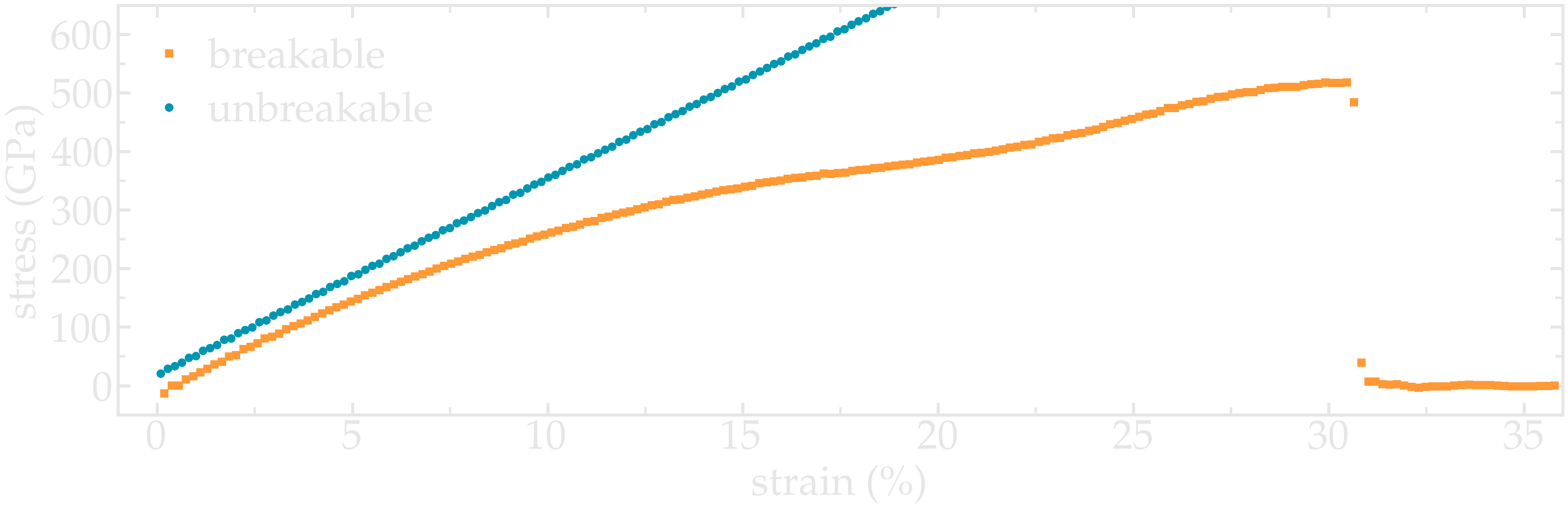
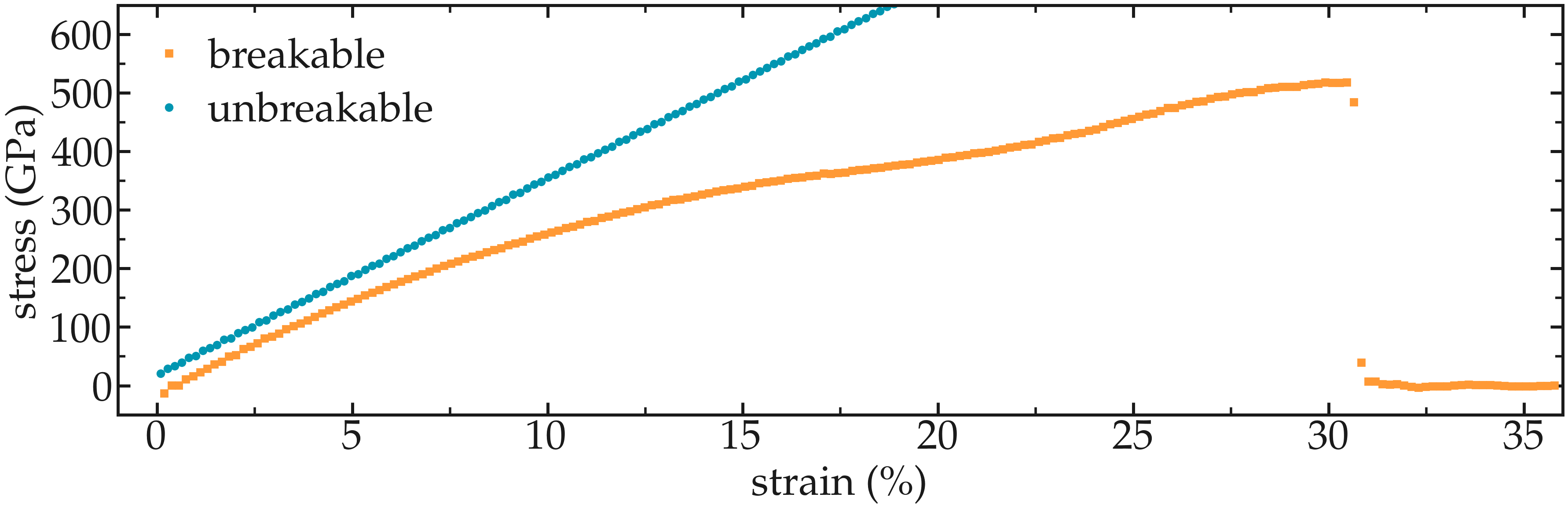
Figure: Strain-stain curves for the two CNTs, breakable and unbreakable.
Solve the flying ice cube artifact
The flying ice cube effect is one of the most famous artifacts of molecular simulations [20]. Download this seemingly simple input, which is a simplified version of the input from the first part of the tutorial. Run the input with this data file and this parameter file.
When you run this simulation using LAMMPS, you should see that the temperature is very close to \(300\,\text{K}\), as expected.
Step   Temp        E_pair      E_mol       TotEng      Press
0      327.4142    589.20707   1980.6012   3242.2444   60.344754
1000   300.00184   588.90015   1980.9013   3185.9386   51.695282
(...)
However, if you look at the system using VMD, the atoms are not moving.
Can you identify the origin of the issue, and fix the input?
Insert gas in the carbon nanotube
Modify the input from the unbreakable CNT, and add atoms of argon within the CNT.
Use the following pair_coeff for the argon, and a mass of 39.948:
pair_coeff 2 2 0.232 3.3952
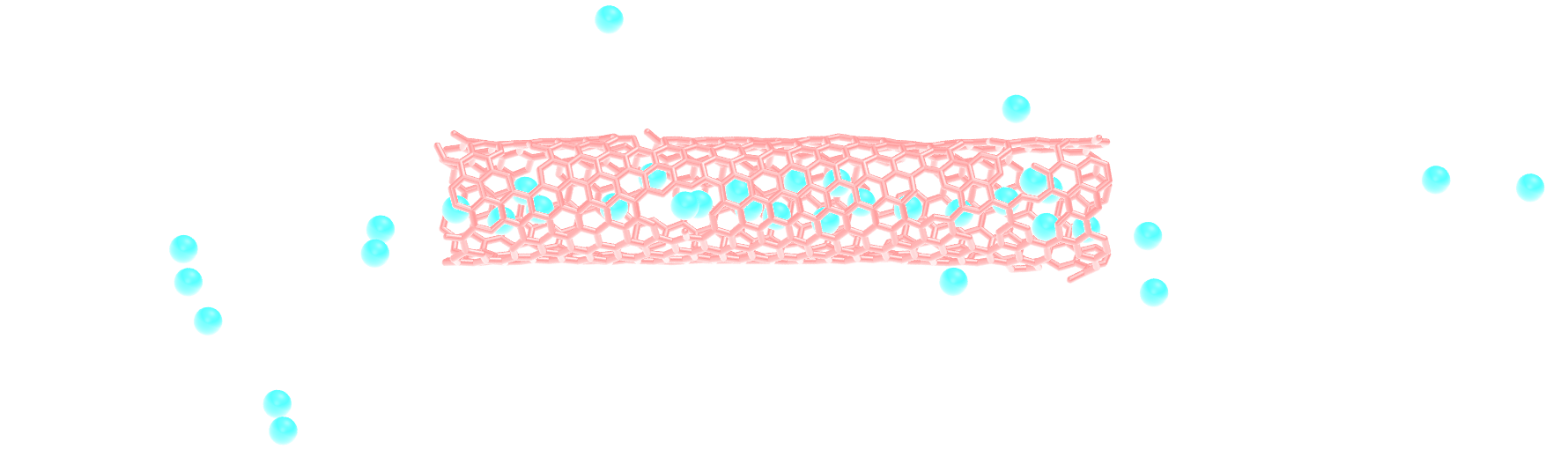
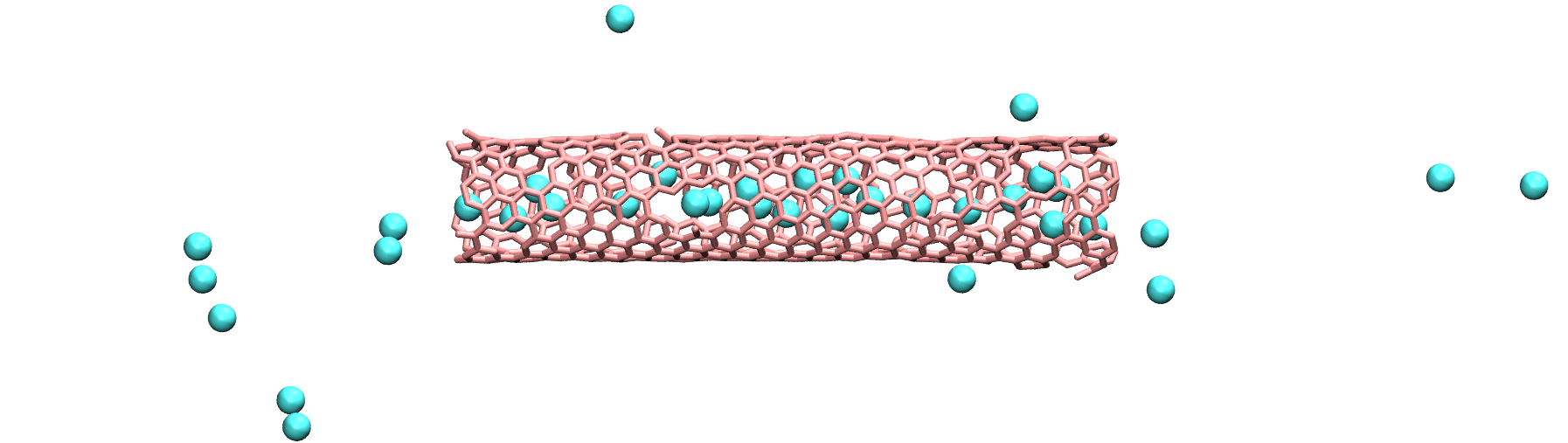
Figure: Argon atoms in a CNT. See the corresponding video.
Make a membrane of CNTs
Replicate the CNT along the x and y direction, and equilibrate the system to create an infinite membrane made of multiple CNTs.
Apply a shear deformation along xy.


Figure: Multiple carbon nanotubes forming a membrane.
Hint
The box must be converted to triclinic to support deformation along xy.