Water adsorption in silica

Adsorption of water in a silica crack using the grand canonical Monte Carlo method

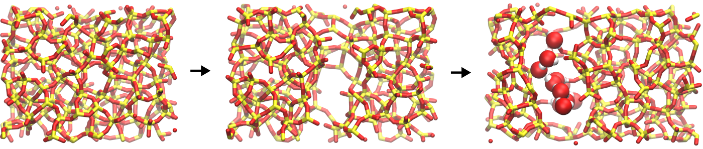
Figure: From left to right: amorphous silica, cracked amorphous silica, cracked amorphous silica with adsorbed water molecules. Silicon (Si) and oxygen (O) atoms of the silica are in yellow and red, respectively, and represented at a network of bonds. The oxygen (O) and hydrogen (H) atoms of the water molecules are in red and white, respectively, and represented as spheres.

The objective of this tutorial is to combine molecular dynamics and grand canonical Monte Carlo simulations to simulate the adsorption of water molecules in a cracked silica, see the figure above. There are three main parts to this tutorial:

• System generation - First, amorphous silica is generated by temperature annealing.
• Cracking - Seconds, the silica is deformed by dilatation of the box until a crack forms.
• Adding water - Third, the system is equilibrated with a water reservoir of given chemical potential using the grand canonical Monte Carlo method.

Generation of the silica block

Let us generate a block of amorphous silica (SiO2). To do so, we are going to replicate a building block containing 3 Si and 6 O atoms. The data file for the SiO atoms can be downloaded by clicking here. Save it in a folder called SilicaBlock. This data file contains the coordinates of the atoms, their masses, and their charges, and can be directly read by LAMMPS using the read_file command. Let us replicate these atoms using LAMMPS, and apply an annealing procedure to obtain a block of amorphous silica.

Create a new input file in the same folder as the downloaded dataSiO.data, and copy the following lines in it:

# Initialization
units metal
boundary p p p
atom_style full
pair_style vashishta
neighbor 1.0 bin
neigh_modify delay 1

# System definition
read_data SiO.data
replicate 4 4 4

Download the Vashishta potential by clicking here.

The system is then replicated four times in all three directions of space.

Then, let us specify the pair coefficients by indicating that the first atom is Si, and the second is O. Let us also add a dump command for printing out the positions of the atoms every 5000 steps:

# Simulation settings
pair_coeff * * SiO.1990.vashishta Si O
dump dmp all atom 5000 dump.lammpstrj

Finally, let us create the last part of our script. The annealing procedure is the following: we first start with a small phase at 6000 K, then cool down the system to 4000 K using a pressure of 100 atm. Then we cool down the system further while also reducing the pressure, then perform a small equilibration step at the final desired condition, 300 K and 1 atm.

# Run
velocity all create 6000 4928459 rot yes dist gaussian
fix nvt1 all nvt temp 6000 6000 0.1
timestep 0.001
thermo 1000
run 5000
unfix nvt1
fix npt1 all npt temp 6000 4000 0.1 aniso 100 100 1
run 50000
fix npt1 all npt temp 4000 300 0.1 aniso 100 1 1
run 200000
fix npt1 all npt temp 300 300 0.1 aniso 1 1 1
run 4000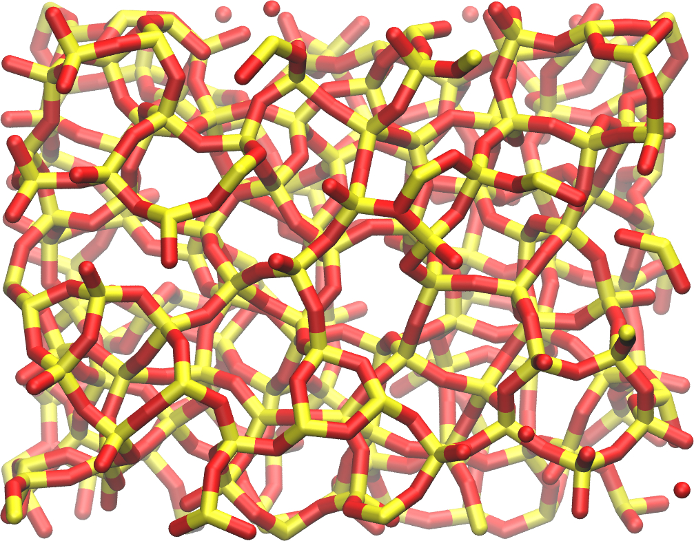
write_data amorphousSiO.data

After running the simulation, the final configuration amorphousSiO.data will be located in the same folder as your input file. Alternatively, if you are only interested in the next steps of this tutorial, you can download it by clicking here. The final system resembles the image below, where the oxygen atoms are in red and the silicon atoms in yellow:

Cracking the silica

We are now going to dilate the block of silica to create a crack. Create a new folder, called Cracking, and create a new input.lammps file starting with:

# Initialization
units metal
boundary p p p
atom_style full
neighbor 1.0 bin
neigh_modify delay 1

# System definition
read_data ../SilicaBlock/amorphousSiO.data

# Simulation settings
pair_style vashishta
pair_coeff * * ../SilicaBlock/SiO.1990.vashishta Si O
dump dmp all atom 1000 dump.lammpstrj

Then, we are going to progressively increase the size of the box over \(z\), thus forcing the silica to crack. To do so, we are going to make a loop using the jump command. At every step of the loop, the box dimension over \(z\) will be multiplied by a factor 1.005. For this step, we use a NVT thermostat because we want to impose a deformation of the volume (therefore NPT would be inappropriate). Add the following lines to the input script:

# Run
fix nvt1 all nvt temp 300 300 0.1
timestep 0.001
thermo 1000
variable var loop 35
label loop
change_box all z scale 1.005 remap
run 2000
next var
jump input.lammps loop
run 20000
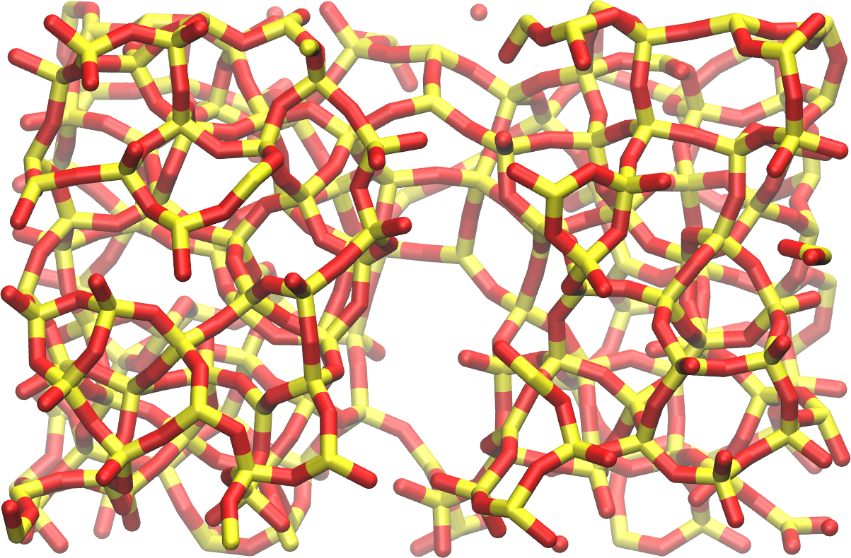
write_data dilatedSiO.data

After the dilatation, a final equilibration step of 20 picoseconds is performed. If you look at the dump file produced after executing this script, or at this video, you can see the dilatation occurring step-by-step and the atoms adjusting to the box size. At first, the deformations are reversible (elastic regime), but at some point, bonds start breaking and dislocations appear (plastic regime). You can download the final state directly by clicking here.

The final system, with the crack, resembles:

Adding water

In order to add the water molecules to the silica, we are going to use the Monte Carlo method in the grand canonical ensemble (GCMC). In short, the system is put into contact with a virtual reservoir of given chemical potential \(\mu\), and multiple attempts to insert water molecules at random positions are made. Attempts are either accepted or rejected based on a Monte Carlo acceptance rule.

In a new folder called Addingwater, add this template file for the water molecule : TIP4P2005.txt. Create a new input file, and copy the following lines into it:

# Initialization
units metal
boundary p p p
atom_style full
neighbor 1.0 bin
neigh_modify delay 1
pair_style hybrid/overlay vashishta lj/cut/tip4p/long 3 4 1 1 0.1546 10
kspace_style pppm/tip4p 1.0e-4
bond_style harmonic
angle_style harmonic

There are several differences with the previous input files used in this tutorial. All these differences are here because this simulation will combine water and silica. First, we have to combine two force fields, vashishta for SiO, and lj/cut/tip4p/long for TIP4P water model. Combining force fields in LAMMPS can be done using the hybrid/overlay pair style. We also need a kspace solver to solve the long range Coulomb interactions associated with tip4p/long. Finally, we need to define the style for the bond and angle of the water molecules. Some of these features have been seen in a previous and simpler tutorial. Before going further, we need to make a few change to our data file. Currently, dilatedSiO.data only includes two atom types, but we need four. Copy the previously generated dilatedSiO.data file within the present folder.

 LAMMPS data file via write_data, version 30 Jul 2021, timestep = 90000

576 atoms
2 atom types

0.910777522101565 19.67480018949893 xlo xhi
2.1092682236518137 18.476309487947546 ylo yhi
-4.1701120819606885 24.75568979356097 zlo zhi

Masses

1 28.0855
2 15.9994

Atoms # full

(...)

We need to make some changes for the addition of water molecules. Modify the file so that it looks like that (the changes are highlighted in bold):

LAMMPS data file via write_data, version 30 Jul 2021, timestep = 90000

576 atoms
4 atom types
1 bond types
1 angle types

2 extra bond per atom
1 extra angle per atom
2 extra special per atom

0.910777522101565 19.67480018949893 xlo xhi
2.1092682236518137 18.476309487947546 ylo yhi
-4.1701120819606885 24.75568979356097 zlo zhi

Masses

1 28.0855
2 15.9994
3 15.9994
4 1.008

Atoms # full

(...)

Doing so, we anticipate that there will be 4 atoms types in the simulations, with O and H of H2O being indexes 3 and 4, respectively. There will also be 1 bond type and 1 angle type. The extra bond, extra angle, and extra special lines are for memory allocation. Now we can continue to fill the input.lammps file, by adding the system definition:

# System definition
read_data dilatedSiO.data
molecule h2omol TIP4P2005.txt
create_atoms 0 single 19.5 10 10 mol h2omol 45585
group SiO type 1 2
group H2O type 3 4

After reading the data file and defining the h2omol molecule from the txt file, the create atoms command is used to include one single molecule in the system at the location 19.5 10 10. I've chosen these 3 values so that the water molecule is initially inside the crack, and not overlapping with SiO atoms, you may have to choose different values. You can estimate these values by looking at your silica structure using VMD. There are cleaner way to do it, such as detecting the free space before inserting the molecule, but for the sake of simplicity, here we are going to do the dirty way here. Not adding a molecule before starting the GCMC steps usually lead to failure. Then, add the following settings of the simulation:

# Simulation settings
pair_coeff * * vashishta ../SilicaBlock/SiO.1990.vashishta Si O NULL NULL
pair_coeff * * lj/cut/tip4p/long 0 0
pair_coeff 1 3 lj/cut/tip4p/long 0.0057 4.42 # epsilonSi = 0.00403, sigmaSi = 3.69
pair_coeff 2 3 lj/cut/tip4p/long 0.0043 3.12 # epsilonO = 0.0023, sigmaO = 3.091
pair_coeff 3 3 lj/cut/tip4p/long 0.008 3.1589
pair_coeff 4 4 lj/cut/tip4p/long 0.0 0.0
bond_coeff 1 0 0.9572
angle_coeff 1 0 104.52
variable oxygen atom "type==3"
group oxygen dynamic all var oxygen
variable nO equal count(oxygen)
fix myat1 all ave/time 100 10 1000 v_nO file numbermolecule.dat
fix shak H2O shake 1.0e-4 200 0 b 1 a 1 mol h2omol
dump dmp all atom 2000 dump.lammpstrj

The force field vashishta applies only to Si and O of SiO, and not to the O and H of H\(_2\)O thanks to the NULL parameters. Pair coefficients for lj/cut/tip4p/long are defined between O atoms, as well as between O(SiO)-O(H\(_2\)O) and Si(SiO)-O(H\(_2\)O). Finally, the number of oxygen atoms will be printed in the file numbermolecule.dat, and the shake algorithm is used to maintain the shape of the water molecule over time. Some of these features have been seen previously, such as in this tutorial.

Let us make a first equilibration step:

# Run
compute_modify thermo_temp dynamic yes
compute ctH2O H2O temp
compute_modify ctH2O dynamic yes
fix mynvt1 H2O nvt temp 300 300 0.1
fix_modify mynvt1 temp ctH2O
compute ctSiO SiO temp
fix mynvt2 SiO nvt temp 300 300 0.1
fix_modify mynvt2 temp ctSiO
timestep 0.001
thermo 1000
run 5000

We use two different thermostats for SiO and H2O, which is better when you have two species, such as one solid and one liquid. It is particularly important to use two thermostats here as the number of water molecules will fluctuate. We use a compute_modify 'dynamic yes' for water to specify that the number of molecules is not constant.

Finally, let us use the gcmc fix and perform the grand canonical Monte Carlo step:

variable tfac equal 5.0/3.0
fix fgcmc H2O gcmc 100 100 0 0 65899 300 -0.5 0.1 mol h2omol tfac_insert ${tfac} group H2O shake shak full_energy
run 250000
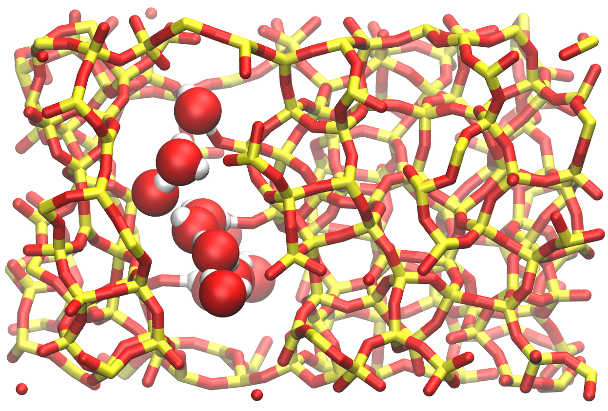
write_data SiOwithwater.data

The tfac_insert option ensures that the correct estimate is made for the temperature of the inserted water molecules by taking into account the internal degrees of freedom. Running this simulation, you should see the number of molecule increasing progressively. Using \(\mu = -0.5\) eV is a reasonable value for the chemical potential that corresponds roughly to ambient conditions (i.e. RH approx 50%).

After 250000 steps, There should be about 10 molecules in the system. This number will vary from one simulation to another, depending on the space available for insertion. The number of molecules also depends on the imposed chemical potential, temperature, and on the interaction between water and silica. The final state looks like this:

Going further

This tutorial is already quite complicated, but if you want to go further, there are several interesting things that can be done with this system:

Relative humidity

You can link the imposed chemical potential with the value of relative humidity (RH). For that, you have to calibrate your simulation by measuring the equilibrium amount of water in an empty box for varying imposed chemical potential, see one of my publication for example.

Isotherm

You can perform a full adsorption isotherm by varying the chemical potential and extracting the equilibrium water content as a function of the imposed RH. Isotherms can be compared to experimental data, and are used sometimes to calibrate force field as it contains a lot of information about the fluid-solid interactions.

Isosteric heat of adsorption

Using the GCMC procedure, you can measure the heat of adsorption by measuring the fluctuations in water molecule and total energy of the system. See this page for details.

Hybrid MD/GCMC

In the grand canonical ensemble, the volume of the box is fixed, so its not possible to capture the swelling of a material with its water content (most material swells with water, like sponges). If you want to model the swelling while also performing a GCMC adsorption simulation, you can alternate between GCMC steps and molecular dynamics steps in the NPT ensemble. This method is called hybrid MD/GCMC.