Graphene sheet and CNT under deformation
Generation of a graphene sheet and a carbon nanotube CNT with VMD, and imposed deformation using LAMMPS
The objective of this tutorial is to use molecular dynamics and simulate the deformation of simple carbon-based structures. There are two main parts to this tutorial:
- Graphene sheet - First, a graphene sheet will be generated using VMD-topotool, and then it will be deformed using an applied displacement (a method called out-of-equilibrium molecular dynamics).
- CNT - Second, a similar protocol will be used to create a single CNT. In this case, a reactive force field will be used, and the breaking of the bonds under extreme deformation will be simulated.
Graphene sheet
Generation of the system
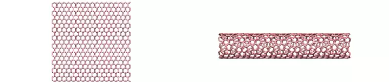
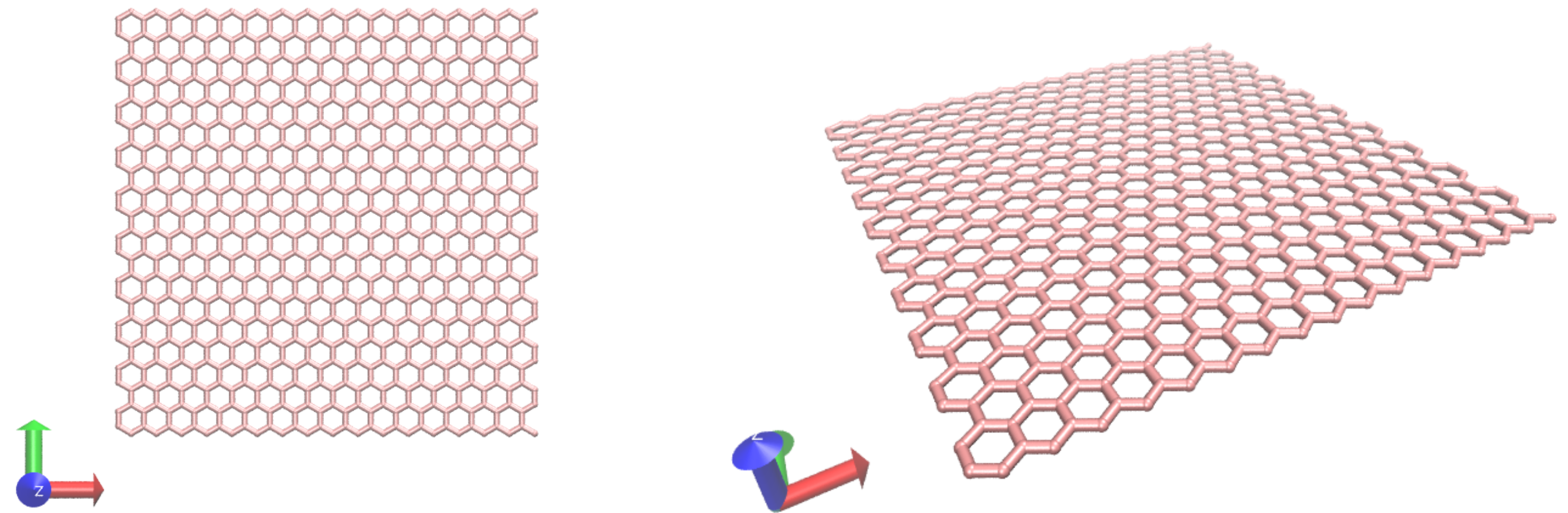
The initial configuration (atoms positions, bonds, angles, etc.) is generated using VMD. Open VMD, and go to Extensions, Modeling, Nanotube Builder. A window named Carbon Nanostructures opens up, allowing us to choose between generating sheet and nanotube of graphene or BN. For this tutorial, let us generate a 4 nm per 4 nm sheet of graphene. Simply change the values of "Edge length along x" and "Edge length along y" to 4, and click on "Generate Sheet(s)". You should see this (here I changed the Drawing Method in Graphics, Representations from Lines to DynamicBonds, and played with the colors, but that is not necessary):
At this point, this is not a molecular dynamics simulations, but a cloud of dots that looks like graphene. In order to generate the initial LAMMPS data file, let us use Topotool and estimate which dots must be connected by bonds using a distance criteria. In the VMD terminal, set the box dimensions by typing the following command in the VMD terminal:
molinfo top set a 80
molinfo top set b 80
molinfo top set c 80
Then, generate the LAMMPS file, enter the following command:
topo writelammpsdata carbon.data fullA new file named "carbon.data" has been created, it starts like that:
LAMMPS data file. CGCMM style. atom_style full generated by VMD/TopoTools v1.8 on Wed Oct 05 19:58:07 CEST 2022
680 atoms
983 bonds
1894 angles
3665 dihedrals
608 impropers
1 atom types
1 bond types
1 angle types
1 dihedral types
1 improper types
-20.965628 59.034372  xlo xhi
-19.438999 60.561001  ylo yhi
-40.000000 40.000000  zlo zhi

# Pair Coeffs
#
# 1  CA
As you can see, the carbon.data file contains information about the positions of the carbons atoms, as well as the identity of the atoms linked by bonds, angles, dihedrals, and impropers constraints.
Save the "carbon.data" file in the same folder as your future LAMMPS input script. We are done with the system generation, we can start the molecular dynamics simulations.
LAMMPS input script
Create a new text file and name it "input.lammps". Copy the following lines in it:
# Initialisation

variable T equal 300

units real
atom_style full
boundary p p p
pair_style lj/cut 14

bond_style harmonic
angle_style harmonic
dihedral_style opls
improper_style harmonic

special_bonds lj 0.0 0.0 0.5

# System definition
read_data carbon.data
Most of these command lines have been seen already in previous tutorials (see this tutorial or this one), with a few differences: first, the pair style here is lj/cut with parameter 14, which means that the atoms closer than 14 Angstroms from each others interact through a Lennard-Jones potential. Notice that there is no Coulombic interaction because all the atoms in pure graphene have a charge of 0. The bond, angle, dihedral, and improper styles specify the different potentials used to restrain the positions of the atoms For more details, have a look at the LAMMPS website (see for example the OPLS dihedral style).
The last command, read_data, imports the carbon.data file previously generated with VMD, which contains the information about the box size, atoms positions, etc.
Parameters for the graphene
Next, we need to specify the parameters of both bonded and non-bonded interactions. Create a new text file in the same folder and name it "PARM.lammps". Copy the following lines in it:
pair_coeff 1 1 0.066047 3.4
bond_coeff 1 469 1.4
angle_coeff 1 63 120
dihedral_coeff 1 0 7.25 0 0
improper_coeff 1 5 180
The pair_coeff sets the Lennard-jones parameters (\(\epsilon\) and \(\sigma\)) for the only type of atom of the simulation: carbon atom of type 1. The bond_coeff provides the equilibrium distance \(r_0\) as well as the spring constant \(K\) for the harmonic potential imposed between two neighboring carbon atoms, where the potential is : \[ E = K ( r - r_0)^2. \] The angle_coeff gives the equilibrium angle \(\theta_0\) and constant for the potential between three neighbors atoms : \[ E = K ( \theta - \theta_0)^2. \] The dihedral_coeff and improper_coeff give the potential for the constraints between 4 atoms. The file PARM.file can be included in the simulation by adding the following line to input.lammps:
include PARM.lammpsSeparate the atoms into 3 groups
The goal of the present simulation is to impose a deformation to the sheet. To do so, we will isolate the atoms of two edges of the graphene sheets into groups, and the displacement will be applied to the atoms of the edge. Add the following lines to the input script :
# Simulation settings

group gcar type 1
variable xmax equal bound(gcar,xmax)-0.5
variable xmin equal bound(gcar,xmin)+0.5
region rtop block ${xmax} INF INF INF INF INF
region rbot block INF ${xmin} INF INF INF INF
region rmid block ${xmin} ${xmax} INF INF INF INF
The first command includes all of the atoms of type one (i.e. all the atoms here) in a group named gcar. Then, two variables are defined: \(x_\mathrm{max}\) corresponds to the coordinate of the last atoms along \(x\) minus 0.5 Angstroms, and \(x_\mathrm{min}\) to the coordinate of the first atoms along \(x\) plus 0.5 Angstroms. Then, 3 regions are defined, and correspond respectively to: \[x < x_\mathrm{min},\] \[x_\mathrm{min} > x > x_\mathrm{max}, ~ \text{and} \] \[x > x_\mathrm{max}.\] Then, let us define 3 groups of atoms corresponding to the atoms located in each of the 3 regions, respectively:
group gtop region rtop
group gbot region rbot
group gmid region rmidThermalisation and dynamics
Let us specify the thermalisation and the dynamics of the system. Add the following lines to input.lammps:
velocity gmid create ${T} 48455 mom yes rot yes
fix mynve all nve
compute Tmid gmid temp
fix myber gmid temp/berendsen ${T} ${T} 100
fix_modify myber temp Tmid
The "velocity create" command gives initial velocities to the atoms of the group gmid, assuring an initial temperature of \(300\,\)K for these atoms. NVE fix is applied to all atoms, thus ensuring that atoms positions are recalculated in time, and a Berendsen thermostat is applied to the atoms of the group gmid only. The "fix modify" ensures that the fix Berendsen uses the temperature of the group gmid as an input, instead of the temperature of whole system. The atoms of the edges are not thermalised because their motion will be restrained in the next part of the input.
Restrain the motion of the edges
To restrain the motion of the atoms at the edges, add the following commands:
fix mysf1 gtop setforce 0 NULL 0
fix mysf2 gbot setforce 0 NULL 0
velocity gtop set 0 NULL 0
velocity gbot set 0 NULL 0
The two setforce commands cancel the forces applied on the atoms of the two edges, respectively, during the whole simulation along \(x\) and \(z\), and the velocity commands set the initial velocities along \(x\) and \(z\) to 0 for the atoms of the edges. Therefore, the atoms of the edges will remain immobile during the simulation (or they would if no other command was applied to them).
Data extraction
Next, in order to measure the strain and stress in the graphene sheet, let us extract the distance \(L\) between the two edges as well as the force applied on the edges. Let us also add a command to print the atoms coordinates in a lammpstrj file every 1000 timeteps:
variable	L equal xcm(gtop,x)-xcm(gbot,x)
fix 		at1 all ave/time 10 100 1000 v_L file length.dat
fix 		at2 all ave/time 10 100 1000 f_mysf1[1] f_mysf2[1] file force.dat
dump 		mydmp all atom 1000 dump.lammpstrj
Notice that the values of the force on each edge are extracted from the fixes setforce 'mysf1' and 'mysf2', by calling them using 'f_', the same way variables are called using 'v_' and computes are called using 'c_'. A fix setforce cancels all the forces on a group of atoms every timestep, but allows one to extract the values of the force before its cancellation.
Run
Let us run a small equilibration step:
thermo 100
thermo_modify temp Tmid

# Run

timestep 1.0
run 5000
With the thermo_modify command, we specify to LAMMPS that we want the temperature \(T_\mathrm{mid}\) to be printed in the terminal, not the temperature of the entire system (because of the frozen edges, the temperature of the entire system is not relevant). Then, let us perform a loop. At each step of the loop, the edges are slightly displaced, and the simulation runs for a short time.
variable var loop 10
label loop
displace_atoms gtop move 0.1 0 0
displace_atoms gbot move -0.1 0 0
run 1000
next var
jump input.lammps loop
What you observe should resemble this video. The sheet is progressively elongated, and the carbon honeycombs are being deformed. You can increase the number of iteration of the loop (variable var) to force a larger elongation.
Carbon nanotube
Using the same protocol as previously (i.e. VMD+topotools), generate a carbon nanotube data file, call it cnt.data. Before generating the CNT, untick "bonds".
Then create a LAMMPS input file, and type in it:
# Initialisation

variable T equal 300

units metal
atom_style full
boundary p p p
pair_style airebo 2.5 1 1

# System definition
read_data cnt.data
The first difference with the previous case (the graphene sheet) is the units: 'metal' instead of 'real', a choice that is imposed by the force field we are going to use (careful, the time is in pico second (\(1\mathrm{e}-12\,\)s) with 'metal' instead of femto second (\(1\mathrm{e}-15\,\)s) with 'real'). The second difference is the pair_style. We use airebo, which is a reactive force field. With reactive force field, bonds between atoms are deduced in real time according to the distance between atoms.
Then, let us import the LAMMPS data file, and set the pair_coeff:
read_data carbon.data
pair_coeff * * CH.airebo C
The CH.airebo file can be downloaded here. The rest of the script is very similar to the previous one:
# Simulation settings

group gcar type 1
variable zmax equal bound(gcar,zmax)-0.5
variable zmin equal bound(gcar,zmin)+0.5
region rtop block INF INF INF INF ${zmax} INF
region rbot block INF INF INF INF INF ${zmin}
region rmid block INF INF INF INF ${zmin} ${zmax}

group gtop region rtop
group gbot region rbot
group gmid region rmid

velocity gmid create ${T} 48455 mom yes rot yes
fix mynve all nve
compute Tmid gmid temp
fix myber gmid temp/berendsen ${T} ${T} 0.1
fix_modify myber temp Tmid
For a change, let us impose a constant velocity to the atoms of one edge, while maintaing the other edge fix. Do to so, one needs to cancel the forces (thus the acceleration) on the atoms of the edges using the setforce command, and set the value of the velocity along the \(z\) direction.
First, as an equilibration step, let us set the velocity to 0.
fix mysf1 gbot setforce NULL NULL 0
fix mysf2 gtop setforce NULL NULL 0
velocity gbot set NULL NULL 0
velocity gtop set NULL NULL 0

variable pos equal xcm(gtop,z)
fix at1 all ave/time 10 100 1000 v_pos file cnt_deflection.dat
fix at2 all ave/time 10 100 1000 f_mysf1[1] f_mysf2[1] file force.dat
dump mydmp all atom 1000 dump.lammpstrj

thermo 100
thermo_modify temp Tmid

# Run
timestep 0.0005
run 5000
At the start of the equilibration, you can see that the temperature deviates from the target temperature of 300 K (after a few picoseconds the temperature reaches the target value):
Step          Temp          E_pair         E_mol          TotEng         Press
0   300           -5084.7276      0             -5058.3973     -1515.7017
100   237.49462     -5075.4114      0             -5054.5671     -155.05545
200   238.86589     -5071.9168      0             -5050.9521     -498.15029
300   220.04074     -5067.1113      0             -5047.7989     -1514.8516
400   269.23434     -5069.6565      0             -5046.0264     -174.31158
500   274.92241     -5068.5989      0             -5044.4696     -381.28758
600   261.91841     -5065.985       0             -5042.9971     -1507.5577
700   288.47709     -5067.7301      0             -5042.4111     -312.16669
800   289.85177     -5066.5482      0             -5041.1086     -259.84893
900   279.34891     -5065.0216      0             -5040.5038     -1390.8508
1000   312.27343     -5067.6245      0             -5040.217      -465.74352
Then. let us set the velocity to 30 m/s and run for a longer time:
# 0.15 A/ps = 30 m/s
velocity gtop set NULL NULL 0.15
run 250000
When looking at the lammpstrj file using VMD, you will see the bonds breaking, similar to this video. Use the DynamicBonds representation.
You can access all the input scripts and data files that have been used in this tutorial from Github.
Going further with exercises
Exercise 1 : Measure the bond length as a function of time
Using the sheet script, extract histograms of the bond length and bond energy as a function of the time.
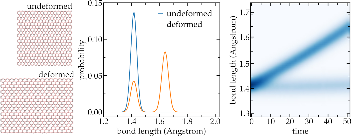
Left: snapshots of the deformed and undeformed graphene sheet. Middle: probability
distribution of the bond length. Right: occurrence of bond length as a function of the simulation time.
50 steps, each increasing the length of the sheet by 0.2 Angstrom have been performed, for
a total elongation of 1 nanometer.
Exercise 2 : Generate a twisted graphene bilayer
Using the sheet script, duplicate the sheet to obtain a bilayer, and rotate one of the sheet, then equilibrate it (without imposed deformation). It should look like this video.
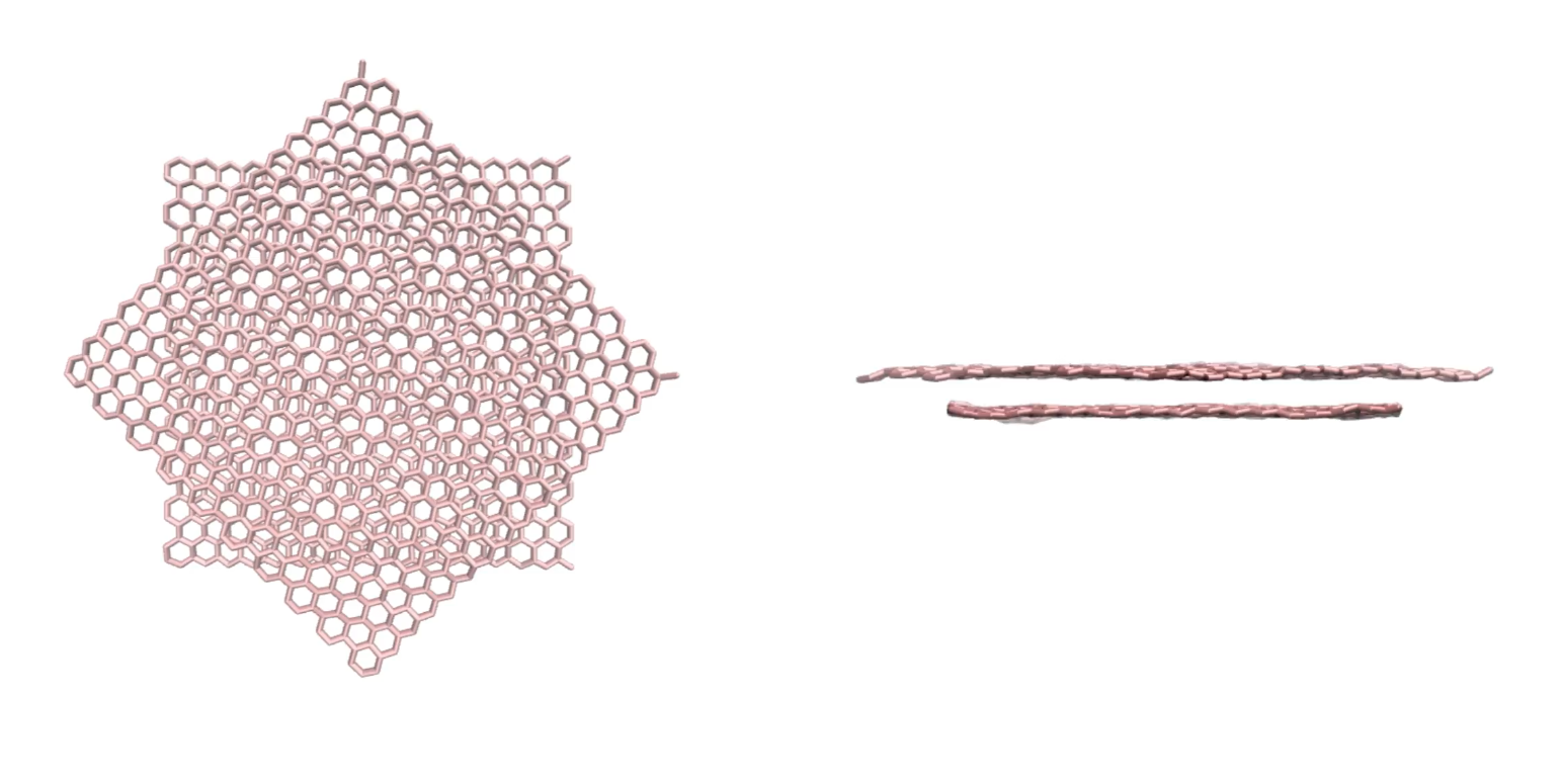
Left: top view of the bilayer. Right: side view of the bilayer.
Exercise 3 : Compress a bulk graphite material
Using the sheet script, makes it periodical over \(x\) and \(y\) directions (i.e. remove the vacuum), duplicate the sheet multiple times along \(z\) and compress it along along \(z\).
Left: graphite at ambient pressure. Right: graphite under a large pressure of 100000 atmospheres applied vertically.